Domestic waste emissions to European waters in the 2010s

The assessment of emissions of nitrogen, phosphorus and organic matter (BOD) in domestic waste involved several steps, namely assessment (i) of the spatial distribution of annual domestic waste (LOCATION); (ii) of the pollution loads (QUANTITY); and (iii) of the level of treatment (REDUCTION).

Location

The Waterbase – Urban Waste Water Treatment Directive (UWWTD) database v6¹⁰, reporting data for 2014, was used as basis for domestic waste emissions in the REP approach region. The UWWTD database reports domestic waste emitted by agglomerations larger than 2000 Population Equivalent (PE) in the 28 European Union Member States plus Iceland, Norway, and Switzerland. The database reports waste loads generated in agglomerations, to which WWTP or IAS loads are transferred to, WWTP treatment levels, and location of WWTP discharge points. All loads are reported in terms of PE. Besides waste generated by resident population, PE loads comprise also commercial, industrial, or tourism waste that is produced in the agglomerations.

The UWWTD database is composed of several tables that portray the complex transfers between agglomerations, WWTPs, and discharge points. The waste load generated in agglomerations may be transferred to WWTPs, to IAS, or discharged without treatment. One agglomeration can be served by more than one WWTP and one WWTP may serve more agglomerations. Similarly, waste from IAS may be released in the environment or transferred in part or in total to one or more WWTPs by truck. Finally, a WWTP may have one or more discharge points.

In the database, some missing data and errors, for example in geographic coordinates, were detected. Further, inconsistencies between waste loads generated by agglomerations, transferred to WWTPs, treated, and ultimately transferred to discharge points were noted. Thus, the original database was amended, filling in missing information where possible and reducing inconsistencies by tracking records through the database structure, with the aim of preserving the generated waste load from agglomerations to treatment facilities and discharge points. Geographic coordinates were corrected where possible based on facility names, or location of linked items (agglomerations, WWTPs or discharge points). Rules applied to address the inconsistencies are detailed in Vigiak et al.¹¹. Not all inconsistencies could be addressed; for example a discrepancy of 10% of waste between what was transferred to and received from any single WWTP was considered acceptable. While the revision process may have reduced database inconsistencies, it may also have inadvertently generated errors, as assumptions had to be made when addressing each inconsistency/error type. This was particularly true for Croatia, for which no information on the path of waste generated in agglomerations to IAS or WWTP was reported, and for which mean statistics of neighbour Slovenia were used instead. Thus, Croatia results should be considered approximations only.

The revision allowed to attribute PE generated in agglomerations (PE_GEN), to IAS or WWTPs discharge points. Waste load treated in IAS (PE_IAS) was equalled to the share of load transferred from agglomerations to IAS (TO_IAS) less the waste load transferred from agglomerations to WWTPs by truck (IAS_to_WWTP; Table 1). In total, about 627.5 million PE were generated in 2014 in the 30 countries comprised in the UWWTD database of the REP region (PE_GEN); of this waste, about 2.3% was not treated (PE_0), 1.8% was treated in IAS (PE_IAS), and 95.9% was connected and treated in WWTPs (PE_WWTP). Due to persistence of small inconsistencies at agglomeration or WWTP level, some small differences between PE generated and allocated to the three waste pathways remained, with the sum of allocations exceeding generated waste by 0.2% overall.

Waste generated in agglomeration but not treated (PE_0) was considered to be discharged directly to the stream network at the agglomeration location, less a 10% abatement that occurs in the sewerage system². As the UWWTD database reports no information about treatment and location of IAS, waste load treated in IAS (PE_IAS) was assumed to receive primary treatment and be discharged in the ground (diffuse source) at the agglomeration coordinates. Waste load treated in WWTPs (PE_WWTP) was reduced according to WWTP treatment level, and emitted in the stream network at the WWTP discharge points. When a WWTP had more than one discharge point, WWTP emissions were divided among discharge points assuming that larger portions of waste would be discharged to larger rivers/streams. The mean annual flow of the receiving reaches was used to define each discharge point receiving fraction.

In parallel and for the whole European continent, domestic waste was also assessed based on national statistics of domestic waste treatment coupled with the spatial distribution of population density (POP approach). This was the only method applicable in the region outside the 30 countries listed in Table 1. The percentage population connected to sewerage system and receiving waste water treatment level were derived from national statistics (Online-only Table 1). The main source of information was Eurostat¹². Population shares were correspondingly defined as: (a) Collected in sewer (%, corresponding to Eurostat ‘Urban wastewater collecting system’); (b) IAS (%, ‘Independent wastewater treatment – total’); (c) 1ary treatment (%, ‘Urban and other waste water treatment plants – primary treatment’); (d) 2ary treatment (%, ‘Urban and other wastewater treatment plants – secondary treatment’); (e) 3ary treatment (%, ‘Urban and other wastewater treatment plants – tertiary treatment’). In a few instances, the distribution in 1ary, 2ary or 3ary treatment plants was unreported in Eurostat¹², but was extracted instead from another Eurostat dataset¹³. From statistics (a) to (e), we derived three more population shares: (f) population whose waste is collected but not treated (Pop_0 = Collected in sewer − sum of 1ary, 2ary and 3ary treatments; = (a) − (c + d + e), %); (g) Disconnected population (DISC), i.e. population share whose waste is not collected in sewers (DISC = 100 − Collected in sewer, = 100 − (a), %); and (h) Scattered Dwellings (SD), i.e. small, sparsely distributed homesteads, equal to the share of disconnected population that is not treated with IAS (SD = DISC − IAS, (g − h) %).

Small inconsistencies in national statistics were identified. For example, IAS data were sometimes unreported or larger than DISC; Pop_0 did not always match Eurostat¹² ‘Percentage of resident population not connected to urban and other waste water treatment plants’ statistics. The inconsistencies were addressed maintaining information about collected and treated shares, i.e. items from (a) to (e), while adjusting derived shares, from (f) to (h). These inconsistencies indicate a degree of conceptual uncertainty in defining population shares or in the interpretation assumed in this study, especially with regards to Pop_0 and DISC. When Eurostat¹² data was not available other reporting sources were used (Online-only Table 1); however it was noted that different international sources indicated sometimes discordant figures¹⁴. Caution should be exerted especially for statistics reported for Albania, Moldova, and Russian Federation.

The 1 km² raster grid of Global Human Settlement (GHS) population of 2015¹⁵ was used to define population density (inhabitants/km²). Population was allocated to waste water treatment shares according to its density, assuming that most densely populated areas would benefit of the best nationally available technology, and vice versa the least populated areas would not be connected to sewerage systems. Thus, four increasing population density thresholds per country were identified based on the national cumulative population density distribution and national treatment statistics as: Th_DISC, below which density of population was assumed disconnected from sewerage; Th₀ defining the density up to which population was assumed to be connected to sewers but whose waste was not treated; Th₁ defining the density up to which population was assumed to be served by primary treatment; and Th₂ defining the density up to which population was assumed to be served by secondary treatment; population densities above Th₂ were assumed to be served by tertiary treatment. After applying the density thresholds, the number of inhabitants per treatment and per catchment was obtained by multiplying the catchment mean density (inhabitants/km²) for the relative share by the catchment area (km²). Through this procedure, population was spatially partitioned into:

1. i.

   Population that is not connected to sewer systems (Pop_DISC: GHS2015 population density < Th_DISC). Pop_DISC was divided in the two fractions, Pop_IAS (i.e. whose waste is treated in IAS) and Pop_SD (i.e. waste generated in scattered dwellings, served by septic tanks). The ratio IAS/DISC between disconnected population whose waste is treated in IAS and all disconnected population was derived from national statistics and used to separate the two fractions: Pop_IAS = IAS/DISC * Pop_DISC; Pop_SD = (1 − IAS/DISC)*Pop_DISC (Online-only Table 1). Thus Pop_IAS and Pop_SD share the same spatial distribution.

2. ii.

   Population that is connected to sewer system but whose waste is not treated (Pop_0: Th_DISC > = density < Th₀)

3. iii.

   Population that is connected to sewer system and whose waste is treated at primary (Pop_1: Th₀ > = density < Th₁), secondary (Pop_2: Th₁ > = density < Th₂), or tertiary level (Pop_3: density > = Th₂).

A final check consisted of summing inhabitants per country and treatment level to see if proportions respected the official statistics. Deviations of allocated to official population shares were less than 0.35% in more than 90% of cases. The largest negative deviation was −3% for tertiary treatment in Turkey, and +3% of primary treatment in Georgia. Within EU28, the largest deviation was +1.2% population allocated to tertiary treatment in Luxemburg. These differences are due to errors in allocating a CCM2 catchment to a single country along country borders.

Merging of domestic waste data sources

The UWWTD database does not report waste from agglomerations below 2000 PE unless its waste is treated in WWTPs. Thus, part of the population that is disconnected from sewerage systems (part of Pop_DISC) or possibly served by sewerage but not treated in small agglomerations (part of Pop_0) remains unreported. To fill in this source gap it was necessary to estimate which quota of population might be unreported in the UWWTD database (called herein “residual population”, Pop_RES). This was done by relating domestic waste estimates from REP and POP approach. However, direct comparison was complicated by (i) differences in reported units, as the UWWTD database reports PE while the POP approach is based on inhabitants; and (ii) the highlighted uncertainties in reported shares of Pop_DISC and Pop_0 for the POP approach.

The relationship between PE reported in the UWWTD database (PE_GEN) and inhabitants (total resident population PopTot, estimated from GHS2015¹⁵) needed be better understood to allow for a meaningful merging of the two approaches. Theoretically, missing population in the UWWTD database would be negligible in countries where shares of scattered dwellings (disconnected but not treated in IAS) or connected but not treated (Pop_0) population is nil or very low. Of the 30 countries analysed in the UWWTD database, 15 reported at least 97.5% of population as treated through IAS or WWTPs (Online-only Table 1). The country ratio between PE_GEN and PopTot (inhabitants) for these 15 countries ranged from 0.8 to 2.4 (median 1.18). Despite this variability and the small sample size, a significant linear regression between PE_GEN and PopTot could be identified: PE_GEN = 1.23 inhabitant (R² = 0.98; sample size = 15; Fig. 2). The rate PE/inhabitant of 1.23 was thus adopted to transform PE into resident population and vice versa. We refer to inhabitants derived from PE as Population Resident Equivalents (PRE, inhabitants), where 1 PRE = 1 PE /1.23. The interpretation of this rate is that on average across Europe the contribution of commercial, industrial and tourism emissions to domestic waste on top of resident population can be considered around 23%. This figure is higher than a global average of 15%² but seems reasonable for industrialized countries, and especially for urban areas.

Fig. 2

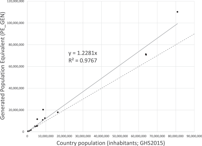
Relationship between generated population equivalent (PE_GEN) as reported in the UWWTD database and total population (inhabitants), for 15 countries that reported at least 97.5% of population as treated through IAS or WWTPs (Online-only Table 1).

Full size image

The PE/inhabitant rate was used to estimate the quota of country population that was not accounted for in the UWWTD database (Pop_RES). Figure 3 shows a conceptual scheme of the procedure. First, country total PE_GEN reported in the UWWTD database (blue bar) was transformed into population resident equivalents (PRE), which were compared to total population (PopTot). The difference between total population (PopTot) and the estimated inhabitants reported in the UWWTD database (PRE) was defined Pop_RES. If the total population was lower than estimated PRE, Pop_RES was nil (case A in Fig. 3). Otherwise (cases B in Fig. 3), Pop_RES was taken (and spatially distributed) as part of population disconnected (Pop_DISC) or connected but not treated (Pop_0). In first instance, if disconnected population was larger than the estimated Pop_RES (case B1 in Fig. 3), then Pop_RES was defined and distributed as the Pop_RES/Pop_DISC fraction of the disconnected population; all this fraction was considered belonging to scattered dwellings (Pop_SD). When Pop_RES was larger than Pop_DISC (case B2 in Fig. 3), then after allocating Pop_SD equal to Pop_DISC, the remaining portion of Pop_RES was taken and distributed as a fraction of connected not treated population (Pop_RES_0). Finally, there could be cases where Pop_RES was larger than the sum of Pop_DISC and Pop_0 (case B3 in Fig. 3). In these cases, all Pop_DISC was considered Pop_SD, all Pop_0 was considered Pop_RES_0, but there was no further attempt to fill the remaining estimated population gap, and the final Pop_RES allocated to the country was lower than the population gap initially estimated.

Fig. 3

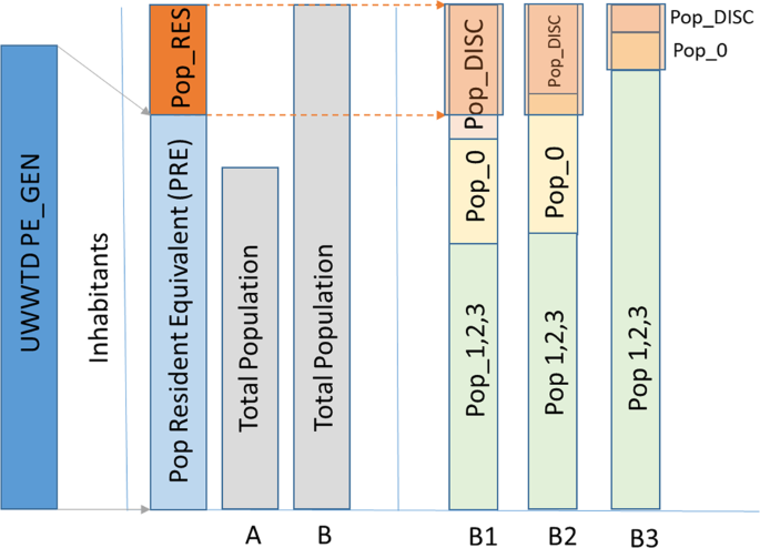
Conceptual scheme of the procedure for assessing population unreported in the UWWTD database (by country) by comparing reported PEs with resident population in the GHS 2015 population dataset. PE_GEN: total generated Population Equivalents per country. PRE: the equivalent amount in Population Resident Equivalent (PRE = PE/1.23; inhabitants). A, B, B1, B2, and B3 represents different cases per European countries (explanation in the text).

Full size image

In some countries (AT, CH, DE, DK, EE, ES, IT, MT, and SE; country codes are indicated in Online-only Table 1), PRE exceeded population thus Pop_RES was nil. In other cases (BE, CY, CZ, LT, LV, PL, SI, and SK), population exceeded PE_GEN; in these countries Pop_RES amounted to 16–42% of population, and was a considerable source of domestic waste in addition to what reported in the UWWTD database. Finally, in the remaining countries (BG, FI, FR, GB, GR, HR, HU, IE, LU, NL, NO, PT, RO) total PE_GEN were larger than population, but the corresponding PRE were lower than population. In these cases, the median Pop_RES was 3% of population, but was larger in FR (9% of population), NO (11%), and FI (17%). In total, Pop_RES amounted to about 25 million inhabitants.

In the POP approach, shares of connected population (Pop_0 to Pop_3) were transformed into PE loads using the PRE equivalence definition, i.e. adding a 23% component due to commercial, industrial and tourism to that of resident population. However, a 10% reduction was applied to these PE loads to account for losses occurring in sewerage system². Pop_IAS were also transformed into PRE, adding a 23% to align them to PE_IAS definition. Instead, domestic load from scattered dwellings (Pop_SD) was considered as produced solely by resident inhabitants (1 PE/inhabitant in this case).

In synthesis, the two datasets (REP and POP) were merged as follows (Fig. 1):

• Treated loads: In regions covered by the UWWTD database, treated load was estimated with the UWWTD database and attributed to discharge point locations (REP approach). For countries not covered by the UWWTD database, treated waste was estimated with Pop_1, Pop_2 and Pop_3 assessed with POP approach, and emissions were distributed according to catchment population density;

• Disconnected and connected not treated domestic loads: In regions covered by the UWWTD database, PE_IAS and PE_0 reported in the UWWTD database were attributed at agglomeration coordinates. Additionally, unreported population pertaining to small agglomerations (Pop_RES) was distributed according to POP approach (Pop_SD and Pop_RES_0). For countries not covered by the UWWTD database, the analogues from POP approach (Pop_SD, Pop_IAS, and Pop_0) were used.

Domestic pollutants loads (QUANTITY)

All waste generated by these sources was considered domestic, although urban waste reported in the UWWTD database includes waste from commercial, industrial, and tourism activities. After allocating domestic waste load (PE) spatially across Europe, the associated emissions of nitrogen, phosphorus, and BOD loads were estimated assuming them to be dependent on human diet^1,16,17.

Emissions of nitrogen and phosphorus from human excreta were estimated based on protein consume¹⁶. Consume was considered equal to intake less a 20% of retail losses for vegetable proteins and 11% for animal proteins, and a further 3% of losses through sweat/hair/blood². Therefore, N and P emissions (E_N and E_P; g/day/PE) were calculated according to Jönsson and Vinnerås¹⁶ as:

where VEGPRT is the vegetable protein intake, ANIMPRT is the animal protein intake (g/day/PE); α_Ν is content of nitrogen in proteins (0.11) and α_P is the content of phosphorus in proteins (0.011)¹⁶. Protein intake was derived from FAO statistics of 2009–2011¹⁸. Emissions of BOD (E_BOD) were assumed equal to 60 g/day/PE as per UWWTD database definition, although BOD emissions in Europe may vary from 40 to 70 g/day/PE depending on diet³. Finally, daily emissions were transformed into annual loads (Load_in,X, t/y):

where X indicates the constituent (nitrogen, phosphorus or BOD). An additional source of phosphorus emissions in domestic waste due to use of detergents was estimated with Bouraoui et al.¹ (Online-only Table 1).

Treatment pollution removal (REDUCTION)

Annual load emissions of domestic waste were computed as:

where Load_out,T,X is the annual pollutant emission load of constituent X (t/y of nitrogen, phosphorus, or BOD) at treatment level T; Load_in,T,X is the annual load undergoing treatment, and eff_T,X is the removal efficiency. Removal efficiencies per treatment level were adopted from literature^3,19,20,21 (Table 2). BOD efficiencies were set after calibration of BOD fluxes in Europe²² within the range of literature values.

WWTP treatment types are reported in the UWWTD database¹⁰, however only nutrient removal technologies were considered to assign tertiary treatment level. WWTP treatment levels for nutrient were thus assigned as follows: tertiary when nitrogen or phosphorus removal was indicated; secondary when secondary treatment was specified, primary in all other cases. Noteworthy, in this way primary level was assigned to 1424 WWTPs which had no treatment reported in the UWWTD database, and to further 394 WWTP ambiguous cases.

Phosphorus removal technology improves tertiary treatment P efficiencies sensibly (T3P; Table 2). In the UWWTD database adoption of phosphorus removal is specified. In the POP approach, national statistics report this information partially¹². However, the fraction of tertiary WWTPs that include phosphorus removal in the UWWTD database was generally higher than Eurostat¹² data, possibly because the UWWTD database is more recent. Thus the rate of phosphorus removal adoption in tertiary treatment (T3P/T3) as estimated from UWWTD database was adopted to define the fraction of Pop_3 treated with phosphorous removal (Pop_3P = Pop_3*T3P/T3). In countries not covered by UWWTD database, for which no data was available, all tertiary treatment was considered without phosphorus removal technology (T3 only; Pop_3P = 0).

Source: Resources - nature.com