General approach
To produce fine-grain climate velocity measures, we modelled monthly temperature and precipitation data averaged for the period from 1981 to 2010 at a resolution of 50-m, incorporating the physiographic effects of solar radiation and cold-air pooling. Based on these data, we calculated estimates for the annual temperature sum above 5 °C (growing degree days, GDD, °C), the mean January temperature (TJan, °C) and the annual climatic water balance (WAB, the difference between annual precipitation and potential evapotranspiration; mm) for our 50-m grid system covering Finland and the adjacent areas (Supplementary Fig. 1S). To investigate how the data resolution affected the velocity measures, 50-m resolution climate surfaces of the three variables were spatially mean-aggregated to a 1-km resolution. For both resolutions, similar future climate surfaces were produced using an ensemble of 23 global climate models from the CMIP5 archives for the years 2070–2099 and the three RCP scenarios (RCP2.6, RCP4.5 and RCP8.5)26. Then using climate-analog approach3,4,9, we measured climate velocities for each of the 50-m and 1-km grid cells based on the distance between climatically similar cells under the baseline and the future climates. In the final step, velocity values were averaged for the focal 5,068 Natura 2000 PA sites to examine their climatic exposure and to assess the overlap between the current and future range in topoclimatic conditions in the PAs.
High-resolution climate data
We developed monthly average temperatures (1981–2010) over the study domain at a spatial resolution of 50 × 50 m by building topoclimatic models based on data sourced from 313 meteorological stations (European Climate Assessment and Dataset [ECA&D])27. The station network and modeling domain covered Finland with an additional 100 km buffer, but it was also extended to cover parts of northern Sweden and Norway for areas >66.5°N (Supplementary Figs. 1S and 2S). This was done because under the current climate changes, future climate spaces similar to the present climate in Finland may be found outside the country borders. Capturing the analogical climate space in areas beyond the country borders is essential in order to avoid developing a large number of velocity values deemed as infinite or unknown. This is especially important in the approach applied in the study, i.e. measuring climate change velocity with the climate-analog velocity approach4,9. In total, our modeling domain constitutes nearly 50 million grid cells.
The methodology to produce the average air temperature data is fully described in Aalto et al.18, and thus only briefly explained here. For temperature modelling we applied generalized additive modeling (GAM) as implemented in the computer software R-package mgcv version 1.8–728,29, utilising variables of geographical location (latitude and longitude, included as an anisotropic interaction), topography (elevation, potential incoming solar radiation, relative elevation) and water cover (sea and lake proximity). A leave-one-out cross-validation suggested that our modelled monthly average air temperatures agreed well with the observations, with the root mean squared error (RMSE) ranging from 0.37 °C (July) to 1.49 °C (January; Supplementary Fig. 3S).
To produce gridded average annual precipitation data (1981–2010), we used global kriging interpolation based on the data from 343 rain gauges obtained from the ECA&D dataset (Supplementary Fig. 2S), geographical location, topography (elevation and eastness index) and proximity to the sea. Kriging interpolation was done using R package gstat version 1.1–030. The eastness index was obtained from a sine-transforming aspect raster surface calculated from a 50 m × 50 m digital elevation model to capture the effect of westerly winds (the prevailing wind direction in the region) on the accumulated precipitation on windward slopes in mountainous areas. To ease the computational burden of the kriging procedure, the gridding was run at a resolution of 500 × 500 m. This was also justified as we expected the annual average precipitation to mainly reflect large scale orographic features, and thus not to significantly vary across short geographical distances. After this, the gridded annual precipitation was bilinearly interpolated into the same 50 × 50 m resolution as the air temperature data. A leave-one-out cross-validation was conducted over the gauge data and indicated a reasonable agreement between the measured and interpolated average annual precipitation sum with an RMSE of ca. 93 mm (Supplementary Fig. 4S).
Bioclimatic variables
Three bioclimatic variables: the annual temperature sum indicating the accumulated warmth (growing degree days, GDD, °C); the mean January air temperature (TJan, °C); and the climatic water balance (WAB, mm) were calculated from the high-resolution gridded climate data (Fig. 1). We focused on these three bioclimatic variables because several earlier species – climate modelling studies have employed same variables and demonstrated their ecological relevance to a large number of habitats and species from different taxonomical groups inhabiting northern environments22,31,32,33,34,35,36. Taken together, these three variables effectively complement each other by providing estimations of winter cold, seasonal warmth and moisture availability which are among the key drivers of biodiversity in our study region. For example, GDD determines the reach of maturity, blooming and completion of life cycle in plant species and the development threshold of insect larvae, the mean temperature of January affects the overwintering survival of species, and the climatic water balance determines the moisture availability for both plant and animal species and the level of drought stress.
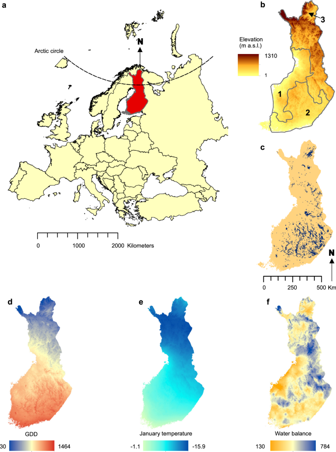
The study area and geographic variation of five environmental variables. (a) Location of the study area in northern Europe. (b) Elevation (m a.s.l.), and three main topographic relief regions in mainland Finland (1 = flatlands; 2 = gently undulating hilly terrain; 3 = rugged terrain with notable variation in elevation), (c) lakes, (d) growing degree days (base temperature 5 °C; GDD), (e) mean January temperature (°C), (f) climatic water balance (mm, difference between annual precipitation sum and potential evapotranspiration). (d–f) Represent average conditions over 1981–2010, modelled at a resolution of 50 × 50 m.
GDD represents the effective temperature sum above the base temperature of 5 °C37:
$$GDD5={sum }_{i}^{n}({T}_{i}-{T}_{b}),,if,{T}_{i}-{T}_{b} > 5$$
where Ti denotes the mean temperature at day i, Tb represents the base temperature, and n is the length of the summation period. Since the daily air temperature data was not available, we estimated the GDD using monthly data following Araújo and Luoto38. The WAB is the difference between the total annual precipitation sum and the potential evapotranspiration (PET), which was estimated from the monthly air temperatures following Skov and Svenning39:
$$PET=58.93times {T}_{above{0}^{^circ }C}/12$$
Coarse resolution climate data
To investigate how the climate data resolution affects the derived climate velocity measures, the high-resolution (50 × 50 m) climate surfaces were spatially aggregated onto a 1 × 1 km resolution grid using an areal mean function. Additionally, although spatially comprehensive, our study domain does not cover parts of western Russia which are adjacent to NE Finland, and which could be a direction for the escaping climates in the future40. Because data and computational constraints prevented us from realistically expanding the topoclimate modeling domain further eastward from the 100 km buffer zone depicted in Supplementary Fig. 1S, the E-OBS data set (version 17.0; 25 km × 25 km)41 covering the areas of ca. 30–50°E were employed, where necessary, to complement the climate velocity analyses for TJan.
Global climate model data
To develop data on future climates, we used the climate projections for the twenty-first century based on an ensemble of 23 global climate models (GCMs), as available from the Coupled Model Intercomparison Project phase 5 archives26. These data were processed to represent the predicted averaged changes in mean temperature and precipitation (with respect to the baseline 1981–2010) over the period of 2070–2099, and three RCP scenarios (RCP2.6, RCP4.5 and RCP8.5)42. The climate model data depicting the predicted change in mean temperatures and precipitation with respect to the baseline climate were bilinearly interpolated onto a matching resolution of 50 × 50 m, and the change predicted by the GCMs was added to the spatially detailed baseline climate data. After this, the bioclimatic variables were recalculated for each RCP scenario to allow the subsequent calculation of climate change velocities and measuring the overlap of the current and future climate ranges within the PAs.
Climate velocity metrics
We calculated the climate change velocities for the three studied bioclimatic variables, GDD, TJan and WAB, using the approach developed by Hamann et al.9, referred to as the distance-based velocity or climate-analog velocity4. In this approach, climate-velocity metrics are calculated by measuring the distance between present-day locations with certain climatic conditions and their future climate analogues, divided by the number of years between the two points in time4. We calculated the climate-analog velocities both for the 50-m resolution grid and the 1-km resolution grid climate data by measuring the distance between climatically similar grid cells for the present and future climates determined by the three climate scenarios, RCP2.6, RCP4.5 and RCP8.5.
Following Hamann et al.9, we selected the boundary values for the classes of bioclimatic variables so that the climatically matching grid cells were defined by setting the within-class range to be as small as possible while, at the same time, avoiding artefactual extreme precision, which could produce unrealistic sporadic patterns in the velocity. To achieve this target, we tested 2–3 different settings for each of the three climate variables and carried out a literature search for earlier class definitions applied to corresponding climate variables. Based on this, the following within-class ranges were selected for the consequent climate velocity analysis: GDD, within-class range 50 °C; TJan, within-class range 0.5 °C; WAB, within-class range 50 mm. The present-day and future climate surfaces of the three climate scenarios were then reclassified by assigning the continuous climate values in each of the 50-m grid cells in one of the 51 GDD, 60 TJan, and 55 WAB categories covering the overall current and future range in the climate space of these variables. This enabled the execution of the search of the minimum distances between grid cells with similar present-day and future GDD/TJan/WAB climates. In technical terms, the search was carried out using the ArcGIS software (Desktop 10.5.1.) by employing the Euclidean distance function. The recommendation by Hamann et al.9 on the “use of gridded data with as high resolution as is computationally feasible and justifiable based on the precision of interpolated climate grids” was achieved in our study by building fine-grained 50-m resolution topoclimatic models, i.e. we used an approach whose methodology and accuracy had been tested in our previous work18.
The resulting measures of the climate velocities for the three climate variables were employed in a series of subsequent analyses. The high-velocity areas (‘velocity hotspots’) of the three climate variables were visually compared with each other based on maps showing their 50-m resolution velocities across the whole of mainland Finland.
Exposure of the protected areas
From the 1,778 protected areas included the Natura 2000 network in mainland Finland we selected 5,068 physically separate Natura 2000 sites (polygons) for this study. Following Nila and Hossein25, we refer to these 5,068 sites as ‘Natura 2000 PAs’, or simply as ‘PAs’. Throughout the European Union, the Natura 2000 network aims to cover the most valuable species and habitats in the 28 member countries (see https://ec.europa.eu/environment/nature/natura2000/index_en.htm). The selection of Natura 2000 PAs was done so that first we dissected each physically separate Natura 2000 PA (i.e. Natura 2000 polygons physically disconnected from other Natura 2000 polygons; e.g. a Natura 2000 area consisting of 5 separate polygons were treated as five individual PAs), then we measured the area of each PA and selected those with a cover of 2 hectares or more. Another selection rule was that from the islands situated close to the coastline of mainland Finland, only PAs on larger islands were included (to avoid the inclusion of smaller islands and islets abundantly surrounded by water areas). For the 5,068 Natura 2000 PAs, we defined the high-velocity PAs (velocity hotspots) as the top 5% showing the highest velocity values. These top 5% high-velocity PAs consisted of 253 sites located in mainland Finland with the highest velocities out of the total of 5,068 PAs. These were assessed separately for the three climate variables, GDD, TJan and WAB, by calculating the mean of the corresponding velocities in the 50-m grid cells included in a given Natura 2000 PA. Based on these data, we assessed in how many of the PAs the velocity hotspots overlapped for two or three variables in the three RCP scenarios (RCP2.6, RCP4.5 and RCP8.5).
Comparison of 50-m and 1-km velocities
The comparisons of the velocity values at the 50-m and the 1-km resolutions were done using only data for the GDD. This was because the velocity patterns for the WAB were rather localised and complex, and because the disappearing climate space in the mean January temperatures would complicate the resolution comparisons in the PAs located in N Finland. The comparisons of the GDD 50-m vs. 1-km resolution velocities in the 5,068 PAs were done in two ways. First, we compared the absolute values of 50-m and 1-km GDD velocity values in each of the 5,068 PAs. For these comparisons, mainland Finland was divided into three relief regions on the basis of the general elevational and topographic features of the terrain (Fig. 1): (i) Relief region 1: flatlands with mostly even terrain (in this region, 10 × 10 km grid squares typically show height differences below 50 m), (ii) Relief region 2: with hilly, undulating terrain varying in height (with typically 50–200 m height differences in 10 × 10 km squares), and (iii) Relief region 3: with rugged terrain and deep valleys or high steeply sloped fell areas (with typically over 200 m height differences in the 10 × 10 km squares). Per-PA comparisons of the absolute differences in the two velocity values were made to assess the number of cases where the 50-m resolution GDD velocity was higher than the 1-km resolution velocity, and vice versa, and to examine the significance of these differences using a paired t-test. These comparisons and tests were done separately for each relief region and each of the three RCPs.
Second, we examined the relative differences between the 50-m and 1-km GDD velocities in the 5,068 PAs. This was done in order to take into account the fact that similar absolute differences in the two velocity values may have a different ecological importance when occurring at different overall levels (e.g. a difference of 0.2 in the velocities very likely matters more between 0.1 and 0.3 than between 2.1 and 2.3). Then, we determined the top 5% of the PAs with largest relative differences between the 50-m resolution and the 1-km resolution velocities and examined how they were divided in the three main relief regions of Finland.
Next, we used generalized linear models (GLMs)43 to test the importance of the relief region, size of the Natura 2000 PA, within-PA elevation range and climate change scenario in explaining the relative differences between the 50-m and 1-km GDD velocities. We fitted a full GLM model where all four explanatory variables were considered at the same time. In this model, relief region was treated as ordinal variables with three levels, the size of the Natura 2000 PA and within-PA elevation range both as log-transformed continuous variables, while the forth variable, climate scenario (RCP2.6, RCP4.5 and RCP8.5), was treated as a categorical factor. Our main interest was in the first three variables (the relief region, the size of the PA and the elevation range within the PA). For these variables, we calculated their effect sizes based on the range between their predicted minimum and maximum values in the observation data while controlling for the influence of other predictors by fixing them at their mean values44.
Overlapping of present-day and future climate spaces in Pas
In addition to the climate velocity analysis, we also examined the degree of overlap between the present-day range and projected future range of the three climate variables in each of the 5,068 Natura 2000 PAs. In order to assess the impact of the data resolution, these analyses were carried out using both the 50-m and the 1-km resolution climate data. Here, we examined whether the fine-grained topoclimate data showed more overlapping between the present-day and the future ranges than the mesoscale 1-km climate data in the PAs. Moreover, in cases where there were not any overlapping parts in the climate spaces, we assessed whether the estimated size of the gap between the present-day and the future ranges depended on the resolution of the climate data. All these assessments were done three times by comparing the present-day within-PA climatic ranges with the projected ranges under the three climate scenarios, RCP2.6, RCP4.5 and RCP8.5. It should be noted that the future within-PA ranges for the GDD and TJan were always either overlapping with the present-day range or located above it, but for the WAB values they overlapped with the present-day range or were located either above or below it (i.e. indicating locally varying, contrasting future changes).
Source: Ecology - nature.com

