Accounting for soil respiration variability – Case study in a Mediterranean pine-dominated forest

Study area

The study area, Pianacci (43°44′31.81″N, 11°06′14.76″E), is a forest stand located about 10 km south of Florence, Italy. The stand is dominated by maritime pine (Pinus pinaster Aiton) and, in suborder, Italian cypress (Cupressus sempervirens L.), with manna ash (Fraxinus ornus L.) and holm oak (Quercus ilex L.) as ancillary species (Supplementary Fig. 2). The climate is typically Mediterranean, with warm and dry summers and relatively cold and wet winters. Data from a weather station 3.5 km away from the study area and referring to the period 1994–2008 accounted for a mean annual precipitation of 764.3 mm, with November as rainiest month (119 mm) and July as the driest (24.4 mm), and a mean annual temperature of 14.8 °C, with January as coldest month (mean 6.5 °C) and July as the warmest (mean 24.2 °C). The terrain is located 216 to 224 m a.s.l. and has a mean slope of 5% and a west to southwest aspect. The soil formed on Oligocene sandstone chiefly composed of quartz, feldspars, and phyllosilicates and somewhere intercalated with thin siltstone layers comprising calcite, quartz, plagioclases, and phyllosilicates. It is a Brunic Arenosol of the World Reference Base for Soil Resources³⁸ and shows an O-A-Bw-BC-C sequence of horizons. Some basic characteristics determined in a soil profile opened approximately in the centre of the stand are shown in Table 3. The very low occurrence of rock fragments in the topsoil (A and B horizons) reveals past agricultural land use.

Monitoring strategy and R_s measurements

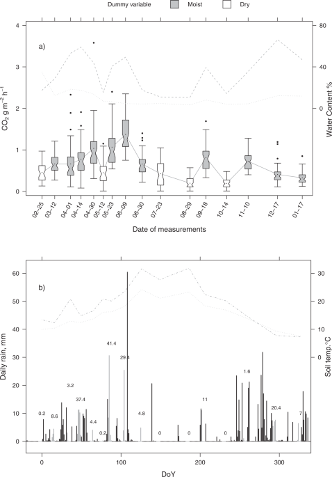
Soil respiration was measured from February 2008 to January 2009, monthly except in April-May-June – the period of highest biological activity – when four extra measurement sessions were carried out (Fig. 1a). The CO₂ efflux from soil was determined by an EGM-1 PP Systems portable gas analyser (Hitchin, UK) coupled with an SRC-1 closed air-circulation chamber 1.17 dm³ in volume. Within a 1/3 ha wide area we selected 50 spots to monitor throughout the year by a randomization procedure, excluding the outermost four-meter-wide strip of the stand to avoid any border effect. Based on the data of Supplementary Tab. 1 such a sampling density was assumed to be high enough to capture most R_s variability and to perform a Bootstrap resampling procedure aimed at finding the minimum number of spots necessary to estimate R_s with an uncertainty close to 10% of the mean of the population.

A stake was driven into the soil 10 cm north of each spot to localize it. We did not place permanent collars into the soil to prevent lateral gas leakage during measurement, as these have been shown to lead to greater underestimation of R_s due to their severing fine roots and the hyphae of mycorrhizal fungi and, possibly, modifying soil temperatures^39,40,41. The R_s measurements were thus carried out by gently inserting the rimmed edge of the chamber 1 cm into the mineral soil and holding the chamber steady during the measurement, to virtually avoid uncontrolled exchanges of air to and from the chamber. At each spot, the temperature of both the atmosphere at ground level and the soil at a depth of 10 cm were recorded. All measurement sessions started at about 11:00, proceeding non-stop in an ordered sequence from spot no. 1 to spot no. 50, which was approximately measured at about 16:00; hence, spending on average about 6 minutes per spot. At each measurement session, two composite samples of both litter layer (O horizon) and top mineral soil were assembled from throughout the area to gravimetrically determine moisture by oven drying at 105 °C to constant mass.

Statistical analysis and model building

In the analysis of data, the CO₂ flux (Y, response variable) was considered: 1) on the original scale; 2) after log transformation; 3) after square root transformation. Explanatory variables were: soil temperature, litter and soil moisture (water % on wet weight). Moisture variables were considered: (a) on the original quantitative scale and (b) after transformation into a binary dummy variable (more details here below). Fitting and examination of linear mixed-effect models were performed following Pinheiro and Bates^42,43. In particular, within each model as in 1), 2), and 3) above-cited points, selection of linear predictors for fixed effects was performed according to BIC (Bayesian Information Criterion) values⁴⁴. In the case of litter moisture, fitted models also took into consideration the above-cited (i) and (ii) alternatives about moisture. Variance heteroscedasticity was considered by introducing random effects associated to sampling dates in all models.

For each best model on the chosen scale of the response (labels 1, 2, 3, above) the analysis of residuals⁴⁵ was done to look for possible evidences of violations in model assumptions. The best models resulting from the above steps were then exploited in the MC simulation.

Litter moisture was found to be a better predictor than mineral soil moisture (Supplementary Tab. 4) and no further improvements of the model came either from the insertion of a cubic parameter or the elimination of the quadratic term (Supplementary Tab. 3).

Whatever the scale for the response variable, the final model matrix X after selecting the best model refers to the following fixed effects: (i) Moisture, defined as in labels (a) and (b) above; (ii) Soil Temperature and its square; (iii) the first order interaction term: Moisture * Soil Temperature, and (iv) Moisture * Soil Temperature².

The matrix Z for random effects has the following hierarchical structure: (i) Sampled Spot and (ii) Soil Temperature within Sampled Spot.

Thus, the expected value of the response is:

The random part of the model defines an intercept at a given date, which is randomly shifted from the value taken in the fixed part of the model. Random fluctuations of the coefficient for soil temperature are also introduced within the sampling date. Such random effects are normally distributed with null expectation. A variance parameter was introduced at each sampling date, so that the variance-covariance matrix of residuals was diagonal but not constant.

Models for transformed responses (labels 1, 2, 3) were adopted with the aim of checking the assumption of normality. A binary dummy variable (label a) was obtained by the sum of the daily precipitations of four days before the sampling date (cp, cumulative precipitation); hence, if cp was less than 0.5 mm, the dummy variable was set to Dry, otherwise it was set to Moist. The “dry” dates were identified at first on an empirical basis, i.e., as those where low values of both litter moisture and R_s were observed, namely 02–25, 05–12, 07–23, 8–29, and 10–14 (Fig. 1a). Sampling dates were those in which the cumulative precipitation was lower than 0.5 mm in the four previous days. Of course, using values other than 0.5 mm and 4 days, different “dry” dates resulted.

The combination of the CO₂ flux (as such, log or square-root transformed) with the two variables (litter moisture or the dummy variable) provided six candidate models for MC simulation (Supplementary Tab. 5 and Fig. 1). The analysis of residuals showed evidence of violation in the assumptions in models with non-transformed CO₂ flux as response (Supplementary Fig. 1) and did not indicate any superiority of one model over the others. Therefore, only the four models with log- or square root-transformed underwent Bootstrap re-sampling and MC simulations.

Uncertainty associated with monitoring fewer spots

The uncertainty associated with monitoring fewer spots was evaluated by Bootstrap resampling^46,47. Several Bootstrap runs were performed by progressively decreasing the number of spots (MCspots) down to 5: that is 49, 48, …6, 5. In each Bootstrap run, for a given MCspots value a random sample with replacement was drawn from the complete dataset (thus forming a Bootstrap Sample dataset, BSdataset); a model was fitted on this BSdataset and, if model fitting converged, confidence intervals were recorded. The stopping rule for resampling was 1001 models successfully fitted to Bootstrap samples (without errors due to convergence, aliasing, etc.).

Two main consequences were expected from the reduction of the MCspots value: (i) the failure of convergence during model fitting and (ii) the increase of uncertainty of parameter estimates, as captured by the difference between the two endpoints of the confidence interval (95%). The R software⁴⁸ and its libraries, nlme⁴⁹ and lattice⁵⁰, were used for data entry, model fitting, and MC simulations.

Data availability

The dataset is available at https://doi.pangaea.de/10.1594/PANGAEA.896345

Source: Ecology - nature.com