Community diversity and habitat structure shape the repertoire of extracellular proteins in bacteria

16S rRNA data and taxonomic classification

We collected 11,649 16S rRNA amplification datasets from MG-RAST (last accessed: march 2015). The datasets had very diverse sizes, with an average size of 100,473 sequences per dataset (Supplementary data 1 and Supplementary Fig. 7). We removed those containing non-ribosomal data or less than 2000 sequences. For this, we queried the sequences of each set for similarities to a 16S rRNA profile using SSU-align v. 1.0.1⁵⁶ using the search algorithm and default parameters. SSU-align uses the conserved secondary structure and sequence of SSU rRNA to identify these sequences. A total of 2329 datasets containing less than 85% of sequences matching the 16S profile were regarded as having low quality and were discarded, leaving 9320 datasets for further analysis (Supplementary Fig. 8).

Sequences were aligned against the same structural profile with SSU-align using the search & global_align algorithm, in order to obtain multiple sequence alignments. The multiple alignments were trimmed using trimal v 1.4⁵⁷ using the automated1 algorithm. The resulting trimmed sequences were clustered into redundant groups of 99% identity using the uclust algorithm from usearch v. 9.0.2132⁵⁸. A reference sequence was selected for each redundant group from each dataset, by selecting the closest sequence to the centroid coordinates. We then defined a global catalog of operational taxonomic units (OTU) for the whole dataset by clustering the reference sequences with usearch into reference OTUs of 97% identity. The reference sequences of each OTU were classified taxonomically against the RDP databases⁵⁹ at species level using blastn v. 2.2.26+ with a minimum e-value of 10⁻⁵ and a minimum coverage of the query 16S rRNA of 80%. We discarded the 38% of the reference sequences that could not be classed in a genus.

Diversity indexes

We used the expected number of species (ENS) as a metrics of the alpha diversity of each 16S rRNA dataset⁶⁰. In order to calculate it, we first used the Shannon diversity index (H′):

where (p_i) is the relative frequency of a specific species in the dataset (the number of sequences associated with the species divided by the total number of sequences assigned to species), and R is the number of datasets.

Based on the Shannon diversity, we calculated the ENS as the exponential of the Shannon diversity:

Finally, we calculated the average values of ENS for the set of habitats where a species (i) was identified. This was defined as the average value of ENS across the samples (j) where it’s present:

where Nd_i is the number of datasets where the species was found. In order to avoid biases associated with the over-representation of specific habitat categories, we made 1000 random samples of an equal number of datasets for each category, and calculated each diversity index as the mean of all measurements (the values can be found in Table S2).

Classification of habitats

The 9320 16S rRNA datasets were classified in terms of habitat using a previously defined nomenclature³⁶, in seven main categories (water, sediment, wastewater/sludge, soil, and host-associated), and 21 sub-categories (henceforth called sub-environments) (Supplementary Data 1 and Table 1).

These categories were divided in five broad groups of increasing habitat structure, and we assigned an integer (h) (from 1 to 5) to each one of them using the method of Kummerli et al.³⁰, to which we removed the distinction of freshwater and marine water, and added a category for Wastewater/Sludge. The rationale behind this classification is associated to the habitat fragmentation generated by its structure; unstructured habitats such as water are seen as a continuum, where any solute molecule has the capacitiy to diffuse freely according to its molecular mass, while highly structured habitats (including soil or host-associated), have physical barriers that create microenviroments, preventing the free distribution of molecules. The habitat structure score h was given as follows: natural aquatic, including freshwater and marine environments (h = 1), sedimentary soils from aquatic environments (h = 2), wastewater/sludge (h = 3), soil (h = 4), and host-associated (h = 5).

Bacterial species were assigned a habitat structure score (habSS) according to the dataset (i) where they were identified (Supplementary data 3):

where n_B is the number of 16S rRNA datasets where the bacterial species B was identified (see Genomic data, taxonomic classification and phylogenetic reconstruction on how species were assigned to OTUs), (c_{i,{mathrm{B}}}) is the number of 16S rRNA reads assigned to species B in the dataset i, (T_{mathrm{b}}) is the total number of reads in the datasets associated to species B, and (h_i) is the value of the habitat structure score for sample i.

Finally, 17 species (1% of the total number) were not found in the 16S rRNA data and could not have a score computed from the data. The environmental structure score of these species was attributed from literature data. 10 out of these 17 species were characterized as obligatory symbionts, including species such as Brucella melitensis, Chlamydia psittaci, Dyckeia dadantii, Mycobacterium tuberculosis, Treponema pallidum, Rickettsia felis, or Sulcia muelleri, among others. The other seven species included bacteria isolated from soil (Geobacter lovleyi, Pimelobacter simplex, Solibacillus sylvestris, Streptomyces avermitilis), sea water (Echinicola vietnamensis, Synecococcus sp. WH7803.), or from highly specific environments, such is the case of Kinecoccus radiotolerans, a soil-associated bacterium isolated from nuclear waste-contaminated sediments⁶¹.

Identification of generalists and specialists

The classification of species into generalists and specialists was performed as follows. We first counted the number of different habitat sub-categories where each bacterial species was identified. In order to account for the prevalence of each species in each habitat sub-category, we calculated the average frequency of each species in each sub-category. The final number of habitats (E) was then weighted by the relative frequency of the species in each habitat sub-category, using the formula:

where (F_{i,j}) stands for the average frequency of the species i in the sub-category j.

From the previous equation, we defined four datasets: species in dataset A, henceforth called specialists, includes the species found in the first quantile of the distribution of the number of habitats (E). Within the specialists, Dataset B (host specialists) was defined by those bacterial species in (A) known to have a strict relationship with hosts, according to the literature⁶¹. Dataset C, henceforth called generalists, includes the species found in the last quantile of the distribution. Finally, Dataset D (host-generalists) included the species in C that are found in hosts. We also identified 136 specialist species (889 genomes, 15%) which were only found in one habitat, and which were used as a validation dataset.

Genomic data, taxonomic classification, and phylogenetic reconstruction

We retrieved all the 5775 completely assembled genomes, including 4794 plasmids, available in GenBank RefSeq (Supplementary data 4, last accessed November 2016). We made two filters on this dataset, one on the number of taxa per phyla, another associated with the 16S mapping procedure. First, to have enough statistical signal, we restricted our analysis to phyla with at least 50 sequenced genomes, resulting in 3922 genomes. We then matched the 16S of the genomes to those of the 16S datasets. For each genome, a representative 16S sequence was extracted from the genome and was aligned using SSU-align with the bacterial structural model. The newly aligned representative sequences were manually trimmed at both edges to adjust the size to the 16S rRNA dataset⁶². The sequences were assigned to a species level using the RDP classifier from the RDP database. The assignation was performed using the Lowest Common Ancestor algorithm, which identifies the lowest convergent taxonomic assignation for all the significant hits of each alignment⁶³. Genomes with ambiguous species classification, i.e., classed in several different species with similar confidence levels, where discarded from further analyses, leaving a total of 1104 species and 3817 genomes.

Since the results are controlled for phylogenetic structure, there is no need to remove further phylogenetic redundancy from the datasets. The 16S rRNA alignment containing the representative sequences of the remaining genomes was used to build a phylogenetic tree using IQ-tree⁶⁴, which identified the substitution model GTR+F+I+G4 as the best (based on the Bayesian Information Criterion). Thousand Bootstrap trees were constructed to determine the topology support at each node.

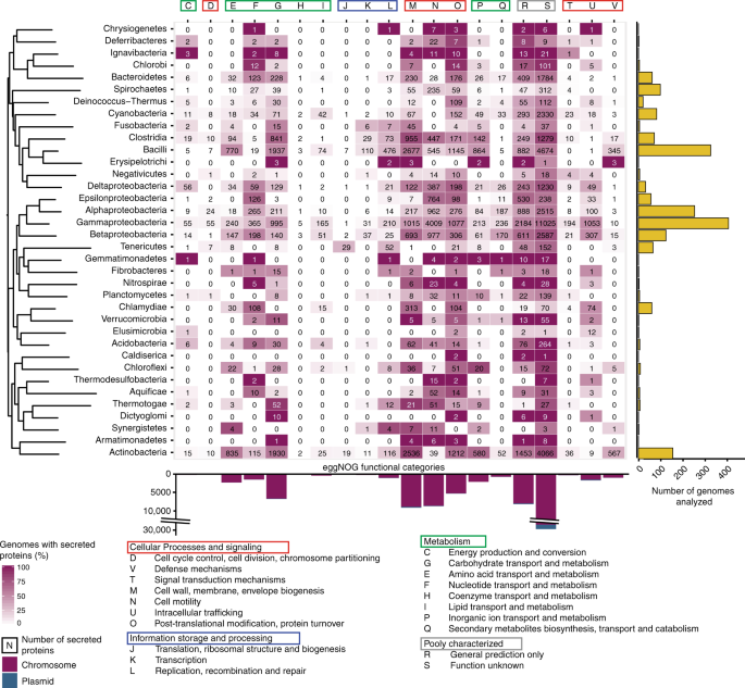
Identification of extracellular proteins, taxonomic, and functional classification

We predicted the sub-cellular location of the proteins encoded in the genomes included in the analysis (see Genomic data, taxonomic classification, and phylogenetic reconstruction) using PSORTB v 3.1²⁹. The PSORTB model was selected based on the species’ monoderm/diderm classification (taken from the literature)⁶¹. Only proteins classified as “extracellular” by PSORTB and lacking transmembrane domains where considered in our study. Proteins not matching these criteria were discarded. When more than one genome was available per species, we computed the average number of proteins per genome for that location (Supplementary data 5). Extracellular proteins were functionally classified by searching for sequence similarity, using HMMsearch from HMMer v.3.1.2b⁶⁵, in the eggNOG v. 4.5 database⁶⁶. We only considered hits with an e-value ≤10⁻⁵ and more than 50% similarity. Since different HMMs may be associated to the same functional category in different taxa, we kept the functional annotation of the best hit when more than half of the hits were associated to that same category (otherwise it was marked unknown).

Three functional categories were explored more carefully. First, we characterized the repertoire of extracellular bacteriocins. To do so, we searched for similarities to the extracellular proteins in the two bacteriocin databases Bagel and Bactibase^67,68 using HMMer. We kept the hits with an e-value < 0.05 and more than 50% coverage of the query sequence (Supplementary Table 2). Second, we identified the extracellular proteins with a degradative activity. We selected enzymatic activities often associated to the extracellular environment: amidase, amylase, cellulase, chitinase, dipeptidase, glycosyl hydrolase, invertase, inulinase, keratinase, and pectinase⁶⁹. For each degradative enzyme, we collected all previously validated bacterial protein candidates by searching for specific keywords in Uniprot1⁷⁰. We clustered them using usearch with the “cluster_smallmem” algorithm at 70% identity. We aligned the sequences of each cluster using mafft v.7 with the local pairwise alignment option and a maximum 1000 iterations (“linsi” option)⁷¹. The resulting multiple alignments were used to build protein HMM profiles using hmmbuild from HMMer. HMM profiles were queried against the extracellular proteins previously predicted. Hits with more than 40% identity and less than 20% difference in length for the smallest of either the protein or profile where kept, and the best hit was used to classify them (Supplementary Table 2).

Quantification of chemical properties of extracellular proteins

We estimated the diffusion length of a protein (d), as in Bard and Faulkner⁷²:

where D is the diffusion coefficient and t the time in seconds.

In aqueous solution, D can be estimated using the Stokes-Sutherland-Einstein equation as proposed by Kalwarczyk et al.⁷³:

where k is Boltzmann’s constant, T is the temperature of the solvent, and η is the viscosity on the solvent. Finally, (r_{mathrm{p}}) is the hydrodynamic radius of a protein, which can be calculated according to its molecular weight (M_w):

We computed the diffusion coefficient for cytoplasm and water, using viscosity values from the literature^74,75. Given the lack of data on the temperatures associated to the environments where the different species could be isolated, we decided to make the simplification that bacteria are in habitats close to their optimal growth temperature ((T_{mathrm{o}})). For each complete genome included in the analysis, we calculated (T_{mathrm{o}}) as in Vieira-Silva et al.⁷⁶.

Extracellular proteins are predicted to be costly because their constituents cannot be recycled easily¹³. To evaluate the effect of the metabolic cost in the environmental distribution, we calculated the biosynthetic cost (in ATP equivalents) per amino-acid for each protein, suing a previously published method⁷⁷ (Supplementary Data 6).

Statistical analyses

We evaluated the phylogenetic effect of the association between the diffusion coefficient of extracellular proteins and the habitat structure, using the R package MCMCglmm³¹. We used the phylogenetic tree of the 16S rRNA sequences as a random factor in the model, according to the package guidelines, with a variance limit to 1. For each analysis, we used 300,000 model iterations with a starting burn-out phase of 50,000, sampling every 100 iterations. From the posterior distributions obtained in this Bayesian analysis, we extracted the (P_{{mathrm{MCMC}}}) (used here as P-value). A low (non-significant, alpha = 0.05) P_MCMC indicates that we cannot exclude the possibility that associations are simply due to phylogenetic structure.

Given the bias towards host-associated habitat datasets in the public repositories, we controlled each correlation test by performing 1000 random samplings of an even distribution of habitats. In all cases, we observed equivalent results for all replicates.

Reporting summary

Further information on research design is available in the Nature Research Reporting Summary linked to this article.

Source: Ecology - nature.com