Collection site
Magdalena Bay is a coastal lagoon on the Pacific coast of the Baja California Peninsula, Mexico, between 25°10′10″N–112°11′24″W and 24°26′24″N–113°33′00″W. Thermal profile data of the sea surface temperature (SST) of the lagoon (Aqua MODIS, NPP, 4 km, daytime, 11 microns, 2003-present, monthly composite) and chlorophyll-a data (mg L) (Aqua MODIS, NPP, L3SMI, global, 4 km, science quality, 2003-present, monthly composite) were obtained for a decade (2006–2016) from the NOAA (National Oceanic and Atmospheric Administration, US). Additionally, in situ SST records were obtained from the culture site (<2 m depth) every 30 min using a HOBO pendant data logger (Onset UA-002-64, US) during April-May (spring) and June-July (summer) 2016 (Supplementary Fig. 1).
Animal sampling and maintenance
N. subnodosus specimens were collected from a suspended culture system (<2 m depth) inside the Magdalena Bay lagoon during the reproductive season previously reported by Arellano-Martínez et al.27. We selected two stages of the annual reproductive cycle in this region: initial development (on May 21st; spring) and advanced development (on July 8th; summer). At each sampling date, sixty scallops were randomly collected, and the gonads of 10 scallops were dissected, and then individually fixed in Davidson’s solution for further histological analysis27. The remaining scallops (n = 50) were carefully placed in a polyurethane box that contained aerated seawater from the culture site and transported to the Centro de Investigaciones Biológicas del Noroeste (CIBNOR) in La Paz, Mexico. During transport (2–3 h), the temperature was monitored using a HOBO data logger (Onset UA-002-64, US) and maintained at 22 ± 1 °C by adding precooled seawater to standardise the transport and acclimatisation temperature on both sampling dates. Upon arrival, the animals were placed in a 150 L water tank and acclimated for eight days at 22 ± 1 °C, under a controlled photoperiod (12 L: 12 D). The water temperature was continuously monitored with a HOBO data logger (Onset UA-002-64, US), while the water salinity (35–36 ppm; Extech Instruments, Waltham, MA, US) and pO2 (90% air saturation; Microx TX2, Presens, Germany) were measured daily. During acclimation, the animals were fed a microalgae diet consisting of Isochrysis galbana and Chaetoceros calcitrans (90,000 cells mL−1, 1:1). The food consumption was monitored daily using a particle counter (multisizer, Beckman, US).
Experimental design and oxygen consumption measurements
The experimental design was partially based on the SST data recorded at the collection site during the spring and summer (Supplementary Fig. 1), which resulted in the scallops being subjected to circadian thermal fluctuations between 19.9 and 25.1 °C and between 20.0 and 27.8 °C one week before the sampling day, respectively. After acclimation, the animals collected each season (spring and summer) were exposed to three experimental treatments: one group was exposed to 22 °C, which is the optimum temperature for juvenile growth26, the second group was exposed to 26 °C, and the third group was exposed to 30 °C, which is close to the upper lethal temperature reported for N. subnodosus juveniles (32 °C)26.
For each experimental group, ten animals were randomly selected, cleaned from epibionts and individually placed in open flow-through glass respiration chambers (60 mL min−1) connected to a header tank, under experimental conditions. The scallops were placed in the chamber at the acclimation temperature (22 °C) and fasted for 12 h before the thermal challenges were started. Water temperature was then gradually increased (1 °C h−1) from the acclimation temperature to one of the two higher target temperatures (26 or 30 °C), after which the temperature was held constant for 24 h. The temperature was continuously monitored using data loggers (Onset UA-002-64, US). Water dissolved oxygen levels were monitored using oxygen microsensors (Microx TX2, Presens, Germany) and were kept above 70% air saturation in all experiments.
Once the target temperature was reached, individual oxygen consumption was measured at 0, 6, 12, 18 and 24 h. The dissolved oxygen levels (% air saturation) were measured using microsensors (Microx TX2, Presens, Germany) connected to the outflow of each chamber (60 mL min−1). A chamber containing an empty shell was used as a blank to correct background respiration caused by microorganisms28. The oxygen microsensors were calibrated at each experimental temperature using Na2SO3 (Fermont, Mexico) saturated water for 0% air saturation and fully aerated seawater for 100% saturation. The oxygen level (percent air saturation) was corrected to the temperature and salinity-specific oxygen capacity of water29. Individual oxygen consumption rates (VO2) were measured for 2 min by switching between animal chambers at each sampling time. The individual oxygen consumption was calculated as follows: VO2 = (ΔVO2 × Vf1)/M, where ΔVO2 is the oxygen consumption of an animal (μmol O2 g−1 h−1) corrected according to the oxygen level in the control respirometer VO2 = (VO2control − VO2animal), Vfl is the flow rate (L h−1), and M is the total soft tissue wet mass (g).
Tissue collection
After 24 h of thermal challenge, the animals were removed from the respiration chambers, and their entire soft tissue biomass was quickly weighed, sampled and immediately frozen in liquid nitrogen. The shells were cleaned, dried, and weighed, after which they were measured with a digital calliper (CD-6CS, Mitutoyo, Japan). The condition index (CI) was calculated as ([total,soft,tissue,wet,weight,(g)/dry,shell,weight(g)]times )(100)30, and the adductor muscle index (AMI) was calculated as ([adductor,muscle,wet,weight(g)/total,soft,tissue,wet,weight,(g)],times 100)30.
Gonadal development
As a quantitative criterion of gonad development, the gonadosomatic index (GSI) was calculated as the percentage of gonad weight to remaining tissue weight rather than total tissue weight using the following formula: (GSI:,[gonads,wet,weight(g)/(total,soft,tissue,wet,weight(g)-)(gonads,wet,weight(g))]times 100), considering that the GSI is affected by changes in mass of either gonadal or somatic tissue as the proportion of gonad wet weight in relation to the total somatic tissue wet weight8. In addition, the gonadal mass index (GMI) was calculated as the proportion of gonad mass in relation to standardised shell height of scallops used in this study (77.55 mm). The allometric relationship between gonad size and body size can be expressed as Y = aHb, where Y is the gonad mass in grams, H is the shell height in millimetres for each season, a is the intercept, and b is the exponent (allometric coefficient), all of which were obtained from log (base 10)-transformed values of gonad mass and shell height to achieve linearity and homogeneity of variances via the following equation: (log ,Y=,log ,a+b,log ,H)31,32.
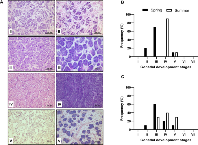
For a qualitative description of gonadal development, histological analysis was performed on 10 scallops collected during both seasons (spring and summer). Each gonad portion was dehydrated via an alcohol series of increasing concentrations (70–100%), cleared with Hemo-De and embedded in Paraplast-Xtra using a microtome, 4 µm-thick sections were obtained and stained with Harris hematoxylin and eosin (H&E) (Humason, 1979) according to histological methods for gonad phases: (I) undifferentiated, characterised by the absence of gametic cells; (II) early development, with expanded follicles and contain oogonia or spermatogonia attached to the follicle wall; (III) late development, characterised by an increase in mature gametes; (IV) maturation (or ripe), with follicles nearly full of free post vitellogenic oocytes in the lumen; V) spawning or partially spawned, with variable quantities of follicles that are partially or totally empty; (VI) spent or post spawning, which corresponds to the recovery phase after spawning; and (VII) resorption, which includes phagocytosis of residual oocytes9,27. Gonadic development images (40X) were obtained using a microscope (Leica DM4B, Germany) connected to a digital camera (Leica, DMC2900, Germany) in conjunction with LAS V software 4.12.
Metabolite extraction and quantification
Frozen samples of adductor muscle were ground to a fine powder with a ball mill mixer (MM400, Retsch, Germany) that was precooled with liquid nitrogen. Nucleotides within the ground adductor muscle samples (100 mg) were extracted and processed according to the methods described by Moal et al.33, with modifications as described by Robles-Romo et al.34. Acidic extracts (200 µl) were neutralised with a mixture of dichloromethane and trioctylamine (5:1 v/v), after which they were passed through a 0.2 µm filter and then maintained at −80 °C until further analysis. The nucleotides were separated by ion-pairing reversed-phase HPLC (model 1100, Agilent Technologies, Palo Alto, CA) with a Hyperclone ODS C18 column (150 × 4.6 mm, 3 µm particle size; Phenomenex, Torrance, CA) connected to a C18 guard column (40 × 3 mm; Phenomenex, Torrance, CA). Separation was carried out in a mobile phase consisting of 0.15 M sodium phosphate monobasic (H2NaO4P), 3 mM tetrabutylammonium (Sigma-Aldrich, Merck, St. Louis, MO) and 8% methanol at pH 6.0, which was adjusted with 5 N NaOH. Nucleotide signals were detected at 254 nm at 0.8 mL min−1 for 22 min. Nucleotide identification was performed using a mixture of standards of ATP, ADP, AMP, GTP, IMP and HX (Sigma-Aldrich, Merck, St. Louis, MO) at known concentrations. The adenylate energy charge (AEC) was estimated according to the methods of Atkinson35 as follows: [(ATP + 0.5ADP)/(ATP + ADP + AMP)].
Arginine phosphate (ArgP) was analysed from the same neutralised extracts used for nucleotide quantification according to the methods of Viant et al.36, with modifications as described by Robles-Romo et al.34 by reversed-phase HPLC in conjunction with a SpheroClone NH2 column (250 × 4.6 mm, 5 µm particle size; Phenomenex, Torrance, CA) connected to a C18 security guard cartridge (40 × 3 mm; Phenomenex, Torrance, CA). The separation was performed at a rate of 1.0 mL min−1 for 18 min in a mobile phase consisting of 0.02 M KH2PO4 buffer (Sigma-Aldrich, Merck, St. Louis, MO) and acetonitrile (72:28) adjusted to pH 2.6 with 5 M H3PO4. ArgP identification and quantification were performed at 254 nm using a commercial standard with a known concentration (Santa Cruz Biotechnology, Santa Cruz, CA). All HPLC-grade reagents were purchased from Fermont, Mexico, and all solutions used were fresh and filtered using a 0.45 µm nylon membrane.
Enzyme activity assays
Activities of metabolic enzymes, hexokinase (HK), pyruvate kinase (PK), cytochrome c oxidase (CCO), citrate synthase (CS), lactate dehydrogenase (LDH), octopine dehydrogenase (ODH), and arginine kinase (AK) were quantified in adductor muscle samples (50 mg) from animals exposed to 22 °C and hyperthermia at 30 °C.
Frozen powder tissue samples were homogenised with specific buffers (1:10, w/v) for each enzyme (Table 1) using a Polytron device (model PT 6100D, Kinematica AG, Switzerland) at 180 g for 30 s at 4 °C and then sonicated (Q125-110, Qsonica Sonicators, Newtown, CT) at time intervals of 10 s (30% output, 4 °C). All samples were analysed during the first hour after homogenisation. Triplicates of each sample were analysed for enzyme activity at 24 °C using a microplate reader (Varioskan Lux, Thermo Fisher Scientific, Finland). Enzyme activity was expressed as units per gram of tissue wet weight (U g−1), where U represents the amount of micromoles of substrate converted to product per minute. All chemicals used were purchased from Sigma-Aldrich Merck, St. Louis, MO. The reaction conditions for the enzyme assays are as follows:
Hexokinase (EC 2.7.1.1): 75 mM Tris-HCl, 7.5 mM MgCl2, 0.8 mM EDTA, 3 mM KCl, 2 mM DTT, 2.5 mM ATP, 1 mM glucose, 0.4 mM NADP, 1 U mL−1 G6PDH, pH 7.3. Abs.: 340 nm. K: 10 min. εNADH = 6.22 mmol L−1 cm−1.
Pyruvate kinase (EC 2.7.1.40): 50 mM imidazole-HCl, 60 mM MgCl2, 2.5 mM ADP, 0.15 mM NADH, 1 U mL−1 LDH, 2.5 mM PEP, pH 7.2. Abs.: 340 nm. K: 14 min. εNADH = 6.22 mmol L−1 cm−1.
Cytochrome c oxidase (EC 1.9.3.1): 50 mM phosphate, 50 µM cytochrome c, pH 7.0. Abs.: 550 nm. K: 10 min. εCyt c = 29.5 mmol L−1 cm−1.
Citrate synthase (EC 2.3.3.1): 100 mM Tris-HCl, 0.1 mM acetyl-CoA, 0.1 mM DNTB, 1 mM oxaloacetate, pH 8.0. Abs.: 412 nm. K: 14 min. εTNB = 13.6 mmol L−1 cm−1.
Lactate dehydrogenase (EC 1.1.1.27): 50 mM imidazole-HCl, 2.5 mM sodium pyruvate, 0.1 mM NADH, pH 6.6. Abs.: 340 nm. K: 10 min. εNADH = 6.22 mmol L−1 cm−1.
Octopine dehydrogenase (EC 1.5.1.11): 50 mM imidazole-HCl, 2.5 mM sodium pyruvate, 3 mM L-arginine, 0.1 mM NADH, pH 6.6. Abs.: 340 nm. K: 10 min. εNADH = 6.22 mmol L−1 cm−1.
Arginine kinase (EC 2.7.3.3): 50 mM imidazole-HCl, 10 mM MgCl2, 10 mM ATP, 1 mM PEP, 0.40 mM NADPH, 1 U mL−1 PK, 1 U mL−1 LDH, pH 7.2. Abs.: 340 nm. K: 14 min. εNADH = 6.22 mmol L−1 cm−1.
Statistical analysis
All variables were analysed for normality (Bartlett test) and homoscedasticity (Levene test). Arcsine and logarithmic transformations were performed if necessary before statistical analysis. One-way repeated measures ANOVA was used to evaluate the effects of thermal challenge (between subjects) over time (within subjects) on the oxygen consumption rate in each season. The Bonferroni test was applied for mean comparisons using the oxygen consumption rate values (control) before the temperature challenge. Two-way ANOVA was used to test the effects of season (spring and summer) and temperature (22, 26 and 30 °C) on nucleotide concentrations and enzymatic activities. Only when a significant interaction was observed individual means for the season plus temperature combinations were compared (Tukey’s HSD test). Otherwise, global means within each factor were compared and indicated in the text. All the statistics and graphics were analysed by Statistica version 7.0 (StatSoft, Tulsa, OK) and GraphPad Prism version 8.0 for Windows (GraphPad, La Jolla CA), respectively. In all cases, statistical significance was accepted at p < 0.05.
Source: Ecology - nature.com

