Origin of Amoebophrya strains and single infected dinoflagellate cells
We based our analyses either on Amoebophrya strains or directly on infected host cells isolated by micromanipulation from environmental samples (hereafter called single-cells). Strains and single-cells were isolated during monitoring for the toxic dinoflagellate species Alexandrium minutum. Monitoring was performed over five years (2007, 2009, 2010–2012) in the Penzé Estuary (48°37′37.57″N, 3°57′13.17″W) and in 2011 in the Rance Estuary (48°31′49.61″N, 1°58′21.81″W), both located in the western Channel (France). Sampling started before the A. minutum bloom (late May-early June) and stopped at the end of the bloom (end of June, beginning of July), generally after 5–7 weeks. Planktonic communities were collected every 1–2 days. For biotic parameters, we fixed cells (>10 µm) with Lugol’s solution and used flow cytometry to count bacteria, viruses, cyanobacteria, picoeukaryotes and phototrophic cryptophytes (based on their pigment and DNA contents). We recorded abiotic parameters including salinity, temperature (air and water), nutrient concentrations (NO3, NH4, and PO4), rainfall and light intensity. Detailed information on the sampling strategy and data acquisition can be found in previously published data focusing on A. minutum blooms9,21,23.
For single-cells, host cells in the late stages of infection by Amoebophrya-like parasites were detected from freshly collected field samples (less than 3 hours) through their natural green autofluorescence using an epifluorescence microscope (BX51, Olympus) equipped with the U-MWB2 cube (450- to 480-nm excitation, 500-nm emission24), then sorted individually by micropipeting, and washed three times into filter-sterilized (<0.22 µm) freshly prepared medium. Hosts were identified according to their morphology, and the single cells were transferred into cryovials with a minimum of medium (3–5 µl), flash-frozen, and stored at −80 °C. DNA extraction and purification were performed both on pelleted strains and single-cells using the MasterPure kit (Epicentre).
To culture Amoebophrya strains, our strategy was to isolate representative phototrophic dinoflagellates, as potential hosts, from the Rance and Penzé Estuaries and other estuaries nearby. We initiated infections in the dinoflagellates by Amoebophrya, either using 3–5 µm filtered samples (fraction presumably containing dinospores) and single, infected dinoflagellate cells (isolated as explained above). Amoebophrya strains were kept in their initial hosts until we reduced the number of hosts to facilitate their maintenance (using either Heterocapsa triquetra or Scrippsiella acuminata STR1). Additional details regarding the isolation and maintenance of strains are described in the supplementary information.
Genome sequencing
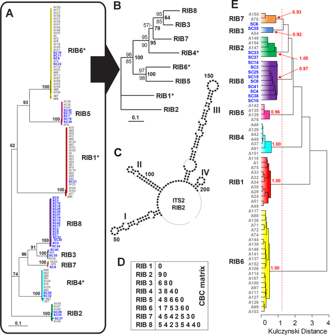
Our strategy to discriminate individuals (i.e., strains and single-cells) was to find fundamental units that formed separate branches on rRNA phylogenetic trees (i.e., ribotypes) and then check whether these fundamental units (or clades) shared a unique combination of phenotypic characters as the backbone for their taxonomy. For that, strains and single-cells were screened by sequencing the ITS1-5.8S-ITS2 region of the ribosomal operon, as explained in Blanquart et al.9. Then, Illumina whole-genome sequencing was performed on a selection of 50 cultivated strains (where the flow cytometry-estimated bacterial contamination was <10%) and 17 single-cells in order to maximize the number of representative Amoebophrya ribotypes. The methodology for cell harvesting for genomic analysis is detailed in the protocole.io dx.doi.org/10.17504/protocols.io.vrye57w. Whole-genome amplification from single-cells was performed using a multiple displacement amplification (MDA) approach with RepliG (QIAGEN, Courtaboeuf, France) according to the manufacturer’s instructions. Paired-end libraries were prepared individually and sequenced on an Illumina HiSeq2000 platform, and a draft genome was assembled for each of the strains. More details regarding sequencing and genome assembly are described in the supplementary information.
Ribosomal operons analyses
We estimated the average number of ribosomal operons per Amoebophrya genome by comparing the read coverage to that of a list of putatively single-copy genes (initial list of 67 genes) (unpublished data). To do so, we first used a BLASTn (e-value < 0.0001) search against the draft genome assemblies to capture the ribosomal operon and the genes of interest. A gene was discarded from the putative single-copy gene list either if i) it was detected in multiple copies using a reciprocal BLAST approach, or ii) had no hit. Genomic reads were then mapped to each of the best hits using Bowtie225. Only the aligned region (i.e., high-scoring pairings as reported by BLASTn) was used for calculating the average coverage of the reference genes and then used to estimate the number of repeated ribosomal operons per genome. In doing so, we used an average of 21 genes per strain (minimum 7; maximum 55).
Compensatory base changes (CBCs)
Full-length ITS2 sequences were directly annotated using Hidden Markov Models (HMMs)26 as implemented in the ITS2 database27 or by alignment to annotated sequences. Secondary structures were predicted by homology modeling using a relevant template (e.g.26,27, or by RNA structure using energy minimization and constraint folding28,29. The phylogenetic analysis of the ITS2 dataset followed the procedures outlined in30. Specifically, a global multiple sequence-structural alignment was automatically generated in 4SALE v1.730,31,32, whereby ITS2 sequences and their respective secondary structures were simultaneously aligned using a 12 × 12 ITS2 sequence-structure specific scoring-matrix33. Phylogenetic relationships were reconstructed by neighbor-joining (NJ) through the use of an ITS2 sequence-structure specific Jukes-Cantor correction (JC) or an ITS2 sequence-structure specific general time-reversible (GTR) substitution model, both implemented in ProfDistS v0.9.934. Using the ITS2 sequence and secondary structure simultaneously (encoded by a 12-letter alphabet33,), a maximum parsimony tree (MP) was reconstructed by PAUP35 based on default settings. A sequence-structure maximum likelihood tree (ML) was calculated using the “phangorn” package36 in R37. Bootstrap support was estimated from 100 replicates. A CBC table was transferred from 4SALE32.
Genome comparison using SIMKA k-mer analysis
We estimated the k-mer distribution of genomes using SIMKA (k = 21 bp; minimum read size ≥90 bp, Shannon index <1.5)38. Due to inherent differences in the genome coverage obtained from cultivated strains and single-cells, we based the cluster analysis upon the presence/absence of k-mers by considering only the distance indexes (based on the formulas given by38) that give more weight to the double presence of k-mers (i.e., Kulczynski, Ochiai, and Chord/Hellinger distances)39. Bootstrap analysis after 100 permutations were obtained using the clusterboot function from the ‘fpc’ R package, directly performed on the distance matrix output by SIMKA with ‘clusterCBI’ as the clustering method, considering the above-estimated number of ribotypes as the desired number of clusters.
Cell phenotype
The rationale for not using morphology and ultrastructure for the characterization of these strains can be found in the supplementary information. Phenotypic characteristics of the strains were deduced from their flow cytometric signatures [i.e., side scatter (SSC), forward scatter (FSC), and natural green autofluorescence], by directly loading 500 µl of fresh cultures on a FACsAria flow cytometer (Becton Dickinson, New Jersey, USA). We additionally estimated the genome size of each strain following the procedure explained in40, where the ratio between the mean distribution of the dinospores and the internal reference Micromonas pusilla RCC299 cells (1 C = 20.9 fg) was used for the evaluation of the nuclear DNA content.
Host range
We determined the host range of the Amoebophrya strains through cross-infection experiments using a diverse selection of locally-occurring dinoflagellate strains isolated from the Rance and Penzé Estuaries and nearby estuarine systems (Table S1, Fig. S2). Freshly produced dinospores were collected by filtration through 5-µm pore-sized cellulose acetate filters (Minisart, Sartorius, Germany) and 100 µl aliquots of this filtrate were inoculated into 1 ml of exponentially growing dinoflagellate strains into 24-well plates. Infections by Amoebophrya strains were detected based on their natural green fluorescence after 2–5 days. Hosts were classified either as resistant (no trace of infection) or sensitive (at least one infected host cell). All cross-infections were processed 3–5 times at different dates.
Environmental metabarcoding survey
We obtained environmental rDNA metabarcoding sequences of 48 samples of the >10-μm size-fraction collected in the Penzé Estuary during late spring and early summer between 2010 and 2012. The DNA was extracted using the phenol-chloroform protocol41, followed by the amplification of the SSU rDNA V4 region (~380 bp) using the universal forward TAReuk454FWD1 primer (5′-CCAGCASCYGCGGTAATTCC-3′), and the modified reverse BioMarKs primer (5′-ACTTTCGTTCTTGATYRATGA-3′)42. PCR amplifications were performed in duplicates for each sample using 5 μM of each primer, 5 μl of 5x buffer, 37.5 mM of magnesium chloride, 6.25 mM of dNTPs, 0.5 unit of GoTaq Flexi (Promega, Wisconsin, USA), approximately 2 ng of DNA (25 μl final volume) and the PCR cycles (initial denaturation: 95 °C for 3 min, 22 to 25 cycles: 95 °C for 45 s, 50 °C for 45 s, 68 °C for 90 s, and final extension: 68 °C for 5 min). The GeT-PlaGe platform (Toulouse, France) performed the Illumina Miseq library preparation and the paired-end sequencing. Taxonomic annotations were performed on unique sequences (100% threshold sequences similarity) observed in at least two different libraries using Mothur43 implemented by the PR2 reference database44 modified to take into account the different ribotypes of Amoebophrya recognized in this study.
Statistical analyses
All the statistical analyses described below were performed in R software using packages freely available on the CRAN repository (http://www.cran-r-project.org).
Comparison of ribotypes based on flow cytometry features, number of operons and host range
We first used Pearson correlations to establish whether the different morphological variables monitored here (excluding host range) were related to one another. Then, differences between ribotypes were assessed by pairwise Mann-Whitney analysis using the cor.test and wilcox.test functions from the basic ‘stats’ package based on [log (x + 1)] transformed data. For comparison of Amoebophrya ribotypes based on their host range, results from the cross-infections were organized into a presence/absence matrix (i.e., infection = 1; no infection = 0) with parasites in the columns and dinoflagellate host strains in the rows. This matrix was then used to generate a heatmap using the function heatmap.2 of the ‘gplots’ package45. Finally, we assessed the relative importance of the phenotypic characters and the host range in the differentiation of the strains belonging to the different ribotypes through a principal coordinate analysis (PCoA) using the cmdscale function of the ‘stats’ package. The PCoA was based on Bray-Curtis distances calculated with the ‘vegan’ package46 from a matrix of descriptors including the standardized values (between 0 and 1) of the phenotypical characters (estimated from their minimum and maximum values47), as well as the presence and absence of infections (1 and 0, respectively) in the different host species. The envfit function of the ‘vegan’ package was used to fit the descriptors to the two first PCoA axes.
Niche analysis
The Outlying Mean Index (OMI) analysis48 was first performed to determine the niche position and niche breadth of Amoebophrya ribotypes using the function niche in the ‘ade4’ package49. We included all 1,153 unique sequences detected in the metabarcodes (distributed into different phylogenetic lineages) to get a better resolution in the niche position of the Amoebophrya ribotypes. Relative read abundances (compared to the total number of reads) and several environmental descriptors [i.e., water temperature, salinity, precipitation, tide coefficient, NO3, PO4 and Si(OH)4] were included in two separate matrixes (N = 48). Before analysis, relative read abundances were Hellinger transformed50 whereas the environmental descriptors were standardized to values between 0 and 147. The function envfit was used to fit the environmental variables to the first two OMI axes. Sample scores from the first two OMI axes were then used to estimate the kernel density weighted by abundance47,48 of Amoebophrya ribotypes using the kde function from the ‘ks’ package51. The niche overlap was then estimated by the comparison of the realized niches (i.e., kernel densities) through the calculation of the D metric52 for each pair of Amoebophrya ribotypes using the ecospat.niche.overlap function from the ‘ecospat’ package53. Pair-wise D metrics were then used to generate a heatmap to detect clustering of the ribotypes related to their niche overlap, following the same procedure described previously for the analysis of the results of the cross-infections.
Relationship between the population fitness of the ribotypes and their host range
We first obtained a more precise estimate of the quantitative contribution of the different ribotypes by dividing the relative abundance of each ribotype in a given metabarcoding sample by their average number of operons estimated from the genome analysis of the strain (hereafter called “normalized abundance). We used the normalized abundances to estimate the population fitness of the six Amoebophrya ribotypes that could be discriminated in the metabarcodes through their V4 sequences, in each one of the three years (N = 18), based on i) their maximal normalized abundances and ii) persistence in the system (e.g., the number of consecutive days in which the non-normalized relative contribution of the ribotype to the total number of reads was higher than 10%). We then determined if these two indicators were different between groups of Amoebophrya ribotypes representing different host ranges (based on the maximal number of infected host species in the cross-infection experiments for each ribotype). This was assessed by Kruskal-Wallis tests using the kruskal.test function in the ‘stats’ package following [log (x + 1)] transformation. In the cases where the Kruskal-Wallis test was significant, the post-hoc Dunn’s test was performed with the dunnTest function in the ‘FSA’ package.
Source: Ecology - nature.com

