Sample fields and crop measurements
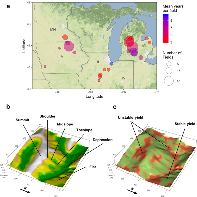
We used yield monitor datasets (i.e., yield maps) for 305 sample fields in Illinois, Indiana, Iowa, Michigan and Minnesota (Fig. 1a). The fields were cropped primarily with corn and soybeans, with a small number also including wheat in rotation. Field size ranged from 10 to 184 ha (34 ha on average), representing a total area of 10,544 ha (Table S1). Each unique field contained at least 3 years of end-of-season yields, collected within 2004–2017. Raw monitor yield data was adjusted to standard grain moisture (15.5% and 13% corn and soybean moisture, respectively) and cleaned as described in a previous study14.
Crop canopy thermal imagery during the month of July were collected at 60 of the fields (Fig. S6a) by a commercial provider (AirScout Inc., Monee, IL, USA) using the aircraft-mounted 9640P thermal sensor (Infrared Cameras Inc., Beaumont, TX, USA). Canopy temperature readings from the thermal band (7–14 µm) were reported as °C (range 12–46 °C) at a 2 m resolution. The georeferenced point-based yield and canopy data were transformed into raster format and resampled to 1-arc second (~30 m) resolution, so that it matched that of the digital elevation model (see below).
For further analysis, we standardized the absolute raster values of yield (Mg ha−1) and canopy temperature (°C) by subtracting the site-year wise mean value and dividing by the standard deviation. In these cases, the standardized values had a mean of zero and standard deviations (σ) as units.
Landscape position classification
For each field, we obtained Digital Elevation Models (DEMs) at 1-arc second resolution (~30 m) from the National Elevation Dataset (NED)38. DEMs were used to calculate local topographic slope and topographic position index (TPI) for each pixel. Topographic slope was computed using the vector-based algorithm39 (i.e., 4 neighbors). Topographic position index (TPI) was calculated with the following equation:
$$TPI={Z}_{i}-{bar{Z}}_{n}$$
(1)
where Zi is the elevation for the ith pixel, and ({bar{Z}}_{n}) is the mean elevation for the surrounding neighborhood. Here, we used a neighborhood of 9 × 9 pixels (~7.3 ha). The computed slope and TPI were used to classify each field pixel into five landscape positions (Fig. 1b): summit (TPI ≥ 1SD), shoulder (1SD > TPI ≥ 0.5SD), midslope (0.5SD > TPI ≥ −0.5SD & Slope ≥ 2%), toeslope (−0.5SD > TPI ≥ −1SD), depression (TPI < −1SD) and flat (0.5SD > TPI ≥ −0.5SD & Slope < 2%), where SD is the standard deviation of TPI values for our entire dataset (0.6 m).
Summit is the uppermost position on a hillslope. It represents a local interfluve, meaning that it receives little overland flow and contributes runoff to downslope positions. The shoulder position is a convex transitional zone at the base of the summit and above the midslope. The footslope lays at the base of hillslopes. Depressions are concave regions that receive most of overland upslope flow. Flat positions show very low local variation in elevation and are not located within sloping terrain.
Temporal stability classification
We followed an established protocol for yield stability analysis40 to partition fields into stable and unstable zones (Fig. 1c). For every pixel of every field, we calculated the mean (µ) standard deviation (σ) of the standardized yields across all the years available for that field. Then each pixel was recoded as stable if σ < 0.75 and unstable if σ ≥ 0.75. Likewise, yield history of each pixel was deemed as low-yielding if µ < 0 and high-yielding if µ ≥ 0. Yield map pixels which had at least one missing value across the different years were excluded from the computation.
Weather and soils
Historical daily weather observations (1988–2017) were extracted for each field from the Daymet dataset41, downscaled to a 1 × 1 km resolution. Daily rainfall and temperature were aggregated to monthly values. Local soil information was retrieved from the Soil Survey Geographic (SSURGO) database42. Each field intersected 2 to 11 map unit polygons, with each map unit including several components. Soil type and properties for the map units’ major components were extracted at each yield map pixel. Then, soil profile data including texture and organic carbon was integrated to 1 m depth for analysis.
Tests of hypotheses
We calculated variance components with hierarchical linear models with all random factors, to quantify the share of the variance in standardized yield (sY) that is accounted by four explanatory variables:
$$sY=mu +{u}_{F}+{u}_{ST(F)}+{u}_{LP(ST(F))}+{u}_{WY(LP(ST(F)))}+varepsilon $$
(2)
where μ is the overall mean, uF is the random effect of field, uST(F) is the random effect of soil type (i.e., SSURGO map unit) within each field, uLP(ST(F)) is the random effect of landscape position within soil type-field combination, uWY(LP(ST(F))) is the random effect of weather year within landscape position-soil type-field combination, and ε is the residual error. The analysis was then repeated by also including yield history as explanatory variable (YH).
To test the hypothesis that yield stability differs among landscape positions, we fitted the following linear mixed effects model to the binomial response of yield stability classification (YSC; i.e., stable or unstable):
$$log ,it(YSC)=mu +{alpha }_{LP}+{u}_{S}+{u}_{S(F)}+{u}_{ST(S(F))}+varepsilon $$
(3)
where αLP are parameters depending on a pixel’s position in the landscape (summit, shoulder, midslope, toeslope, depression and flat), uS is the random effect of state, uF(S) is the random effect of field within state, and uST(F(S)) is the random effect of soil type within field and state. We applied the logit function to generalize the binomial response to a linear model, and back transformed the results using the inverse logit function.
We also tested whether standardized yields in unstable pixels across landscape positions responded differently to May cumulative rainfall (MCR; mm), July cumulative rainfall (JCR; mm), and July mean daily maximum temperature (JMT, °C), using the following model:
$$sY=mu +{alpha }_{LP}ast ({beta }_{1}ast MCR+{beta }_{2}ast JCR+{beta }_{3}ast JMT)+{u}_{F}+{u}_{ST(F)}+varepsilon $$
(4)
where β1, β2 and β3 are regression slope coefficients. Finally, we tested differences in the standardized canopy temperatures (sCT) in unstable pixels among landscape positions:
$$sCT=mu +{alpha }_{LP}+{u}_{F}+varepsilon $$
(5)
Differences among the six levels of landscape position were tested using the Tukey adjustment to correct for multiple comparison. In all tests, we rejected the null hypothesis (i.e., no effect) if the estimated probability was lower than 0.05. All test used the corn and soybean crop years only.
Given similar responses to weather (Fig. 2c), we pooled landscape positions into three classes: upland (summit, shoulder and midslope), lowland (toeslope and depression) and flat. We considered to be areas prone water deficit as those that exhibited unstable yields and were located in the upland position, whereas excess water-prone areas as those lowland positions with unstable yields. Then for every field and year, we computed their mean yield relative to the field-year mean yield.
To estimate yield penalty as a function of seasonal rainfall, we fitted OLS regression to the relative yield in areas prone to excess and deficit water, independently for each zone type and crop, with seasonal rainfall anomaly as the independent variable. This was computed by subtracting the site’s long-term (1988–2017) mean rainfall and scaling by the standard deviation.
We modeled the response of field mean yield ((bar{y})) to seasonal (May—Sep) rainfall using Rickter’s curve43:
$$bar{y}=aast (x-c)ast {exp }(-bast (x-c))$$
(6)
where x is independent variable of seasonal rainfall anomaly, and a, b, and c, are the fitted constants. The models were computed independently for corn and soybean. Finally, we linked the OLS regressions with the non-linear model, so that the idealized response of yield (y′) in drought- or flood prone areas was:
$$y{prime} =({beta }_{0}+{beta }_{1}ast x)ast bar{y}$$
(7)
where β0, and β1 are the OLS regression parameters.
Up-scaling to regional-level impacts
To assess regional-level yield gaps in drought and flood-prone subfield zones and associated impacts, we use a satellite-derived yield stability classification of corn and soybean cropland for 10 Midwestern states13 (Fig. S12). This yield stability classification is based on temporal variability in NDVI derived from Landsat 5, 7, and 8 images (30 m resolution) collected between 2010 and 2017. Details about the image classification procedure, as well as ground-truth validation, are provided by a previous study13. Yield stability classifications were laid over regional NED-DEMs to determine the share of unstable yield zones in upland, lowland or flat areas. Total cropland area and the percentage of cropland in unstable lowland and upland was aggregated for each county. We excluded urban counties (population > 100,000) and those with <1,000 ha under corn or soybean cultivation.
We estimated county-level yields in water-excess and water-deficit prone cropland (y′) for the period 2007 to 2016 using Eq. (7). In this case, (,bar{y}) is the average county yield as reported by the National Agricultural Statistic Service44 (NASS; Figs. S13 and S14), and x is the seasonal (May-Sep) rainfall anomaly for each US climate division (Fig. S15). Monthly rainfall values for each climate division are averages computed using daily observations from individual weather stations. Climate data was accessed through the Iowa Environmental Mesonet Climodat web portal45.
Software
All data processing and analysis was conducted in R (version 3.5.2) extended with the following packages: daymetr to query Daymet data; FedData to access NED and SSURGO databases; sp and raster to process spatial data and terrain analysis; dplyr and tidyr for all other data wrangling; lme4 for linear-mixed effects model fitting; emmeans for post-hoc mean comparison; nlme for non-linear model fitting; and rasterVis and ggplot2 for data visualization.
Source: Ecology - nature.com

