We base our model upon the classical Lotka-Volterra equations23, to which we add a second prey species and combine it with the SIR model24. To simplify the analysis, we assume that the disease is 100 percent fatal, as recovery with immunity would give rise to a number of new steady states and complex scenarios. This model is in part based on an earlier model25, though this had non-linear functional and numerical responses. The older model also exhibits chaotic behaviour, and we will examine it in the supplement.
In order to achieve the most basic system of equations, we assume that all functional and numerical responses are linear, that there is no competition between the prey species, and that there is no carrying capacity on the prey nor the predator. It should however be noted that chaos is still possible in systems with nonlinear functional responses and a prey carrying capacity. We further assume that healthy and infected animals are equally difficult to catch and equally nutritious for the predator. Thus, we arrive at the following equations:
$$begin{array}{rcl}frac{d{x}_{s}}{dt} & = & {alpha }_{x}{x}_{s}-beta {x}_{s}{x}_{i}-{{epsilon }}_{x}{x}_{s}z frac{d{x}_{i}}{dt} & = & beta {x}_{s}{x}_{i}-{{epsilon }}_{x}{x}_{i}z-gamma {x}_{i} frac{dy}{dt} & = & {alpha }_{y}y-{{epsilon }}_{y}yz frac{dz}{dt} & = & {eta }_{x}({x}_{s}+{x}_{i})z+{eta }_{y}yz-delta z,end{array}$$
(1)
where xs and xi are healthy and infected populations of the susceptible prey species, y is the population of the immune prey species, and z is the population of predators. αx,y are the reproduction rates of the prey species, β is the infection coefficient of the disease, and γ is the death rate of infected individuals. Finally, εx,y are the coupling constants signifying the rate of individual prey of species x and y being eaten per predator, while ηx,y are the predator reproduction rates from eating prey of species x and y, and δ is the predator starvation rate in the absence of prey. This is far too many parameters to allow us to get any meaningful information out of the system. Therefore, we rescale it to a timescale and characteristic populations that reflect the dynamics of the system.
First, let (tilde{t}) ≡ γt, meaning that we will measure time in units of the time it takes an infected prey to die. Thus, the lifetime of the disease is our timescale. We also choose the unit of prey population sizes to be the Lotka-Volterra equilibrium populations in a prey-predator system with only that prey species and the predator. The unit of predator population is similarly chosen as the equilibrium predator population in a Lotka-Volterra system with only the susceptible prey and the predator. Finally, the unit population of infected prey is the same as for susceptible prey. This means that ({mathop{x}limits^{ sim }}_{s}equiv frac{{eta }_{x}}{delta }{x}_{s},,{mathop{x}limits^{ sim }}_{i}equiv frac{{eta }_{x}}{delta }{x}_{i},mathop{y}limits^{ sim }equiv frac{{eta }_{y}}{delta }y) and (tilde{z}equiv frac{{{epsilon }}_{x}}{{alpha }_{x}}z.) We then have
$$begin{array}{ccc}frac{d{mathop{x}limits^{ sim }}_{s}}{dt} & = & a{mathop{x}limits^{ sim }}_{s}-R{mathop{x}limits^{ sim }}_{s}{mathop{x}limits^{ sim }}_{i}-a,{mathop{x}limits^{ sim }}_{s}mathop{z}limits^{ sim } frac{d{mathop{x}limits^{ sim }}_{i}}{dt} & = & R{mathop{x}limits^{ sim }}_{s}{mathop{x}limits^{ sim }}_{i}-a{mathop{x}limits^{ sim }}_{i}mathop{z}limits^{ sim }-{mathop{x}limits^{ sim }}_{i} frac{dmathop{y}limits^{ sim }}{dt} & = & bmathop{y}limits^{ sim }-acmathop{y}limits^{ sim }mathop{z}limits^{ sim } frac{dmathop{z}limits^{ sim }}{dt} & = & d({mathop{x}limits^{ sim }}_{s}+{mathop{x}limits^{ sim }}_{i}+mathop{y}limits^{ sim }),mathop{z}limits^{ sim }-dmathop{z}limits^{ sim },end{array}$$
(2)
where a ≡ αx/γ, b ≡ αy/γ, c ≡ εy/εx, d ≡ δ/γ and R ≡ β x(0)/γ = βδ/γηx. R (often called R0 for a given epidemic) is the basic reproduction number of the disease at the initial susceptible prey density xs = 1. The basic reproduction number is defined as the number of new infections caused by one infected individual dropped into a susceptible population. In real epidemics R varies from around 1, the minimum required for the epidemic to start, up to around 18 in extremely infectious diseases such as measles26. This rescaling allows us to reduce the number of unknown parameters from nine to five, and also rids us of the coupling constants ηx,y whose size and relationship with εx,y are hard to determine. From now on, we will drop the tildes and simply use x,y,z etc. to refer to dimensionless variables. With so relatively few parameters, extracting information from the equations should be easy. This is what we will do in the following section.
Stability analysis
If for some parameter values the system has only one stable fixed point, we will intuitively expect it to not be chaotic. Therefore, we should be able to learn more about the potential for chaos in the system by looking at the stability of the fixed points. The physically possible (i.e. where no populations are strictly negative), nontrivial fixed points of the system 2 are
$$(begin{array}{c}{x}_{s} {x}_{i} y zend{array})=(begin{array}{c}1 0 0 1end{array}),(begin{array}{c}0 0 frac{b}{ac} 1end{array}),(begin{array}{c}frac{1}{R} frac{a}{R} 0 0end{array}),(begin{array}{c}frac{b+c}{Rc} frac{ac-b}{Rc} frac{b}{ac} frac{R-1-a}{R}end{array})$$
(3)
For the first fixed point, where the susceptible prey and the predator reach an equilibrium, we have two real and two purely imaginary eigenvalues of opposite sign. The real eigenvalues are (b − ac, R − 1 − a). We expect this fixed point to be (marginally) stable if the real eigenvalues are both negative, i.e. if b < ac and R < 1 + a. This translates into a situation where the disease is infectious enough to spread and the immune prey reproduces slowly relative to the susceptible prey.
The second fixed point, where the immune prey and the predator coexist in a Lotka-Volterra equilibrium, similarly has two conjugate imaginary eigenvalues and two real ones, (−1 − b/c, a − b/c). As b and c are always positive, we expect the first eigenvalue to be strictly negative. The second will be negative and give rise to stability if b > ac, opposite of the other fixed point.
The third fixed point, an analogue to the Lotka-Volterra steady state but with the pathogen replacing the predator, has two imaginary and two real eigenvalues like the others. One of the real ones is c, however, which we know is always positive, so this fixed point is unstable as long as there are two prey species.
Finally, the fixed point with coexistence of all populations has eigenvalues that are the fourth roots of some function of the parameters. As we know that the fourth roots of any number will be four complex numbers at orthogonal angles in the complex plane, their real parts will always have mixed signs, and this equilibrium will be unstable. Our stability analysis shows that there are two stable fixed points in which the system might end up: If the disease is less infectious than some threshhold R < 1 + a, and it holds that the immune prey reproduces slower than the threshhold b < ac, it will end up in the first fixed point, where only the susceptible prey and the predator persist. If the opposite is true, b > ac, the system will end up in the second fixed point regardless of R. Two diagrams of the conditions for stability can be seen in Fig. 2(a,b). On the other hand, if both
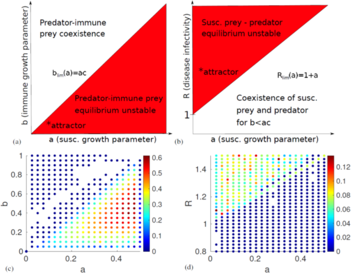
Diagrams of the analytically derived linear stability of the system and the numerical measurements of the Lyapunov exponent. (a) Stability of the predator-immune prey equilibrium as a function of the susceptible and immune prey reproduction parameters a and b. We see that the system will end up in this fixed point if b > ac. (b) Stability of the predator-susceptible prey equilibrium as a function of a and the disease basic reproduction number R. The system will end up at this fixed point if b < ac and R < 1 + a. Thus, we can conclude that chaos is possible only if b < ac and 1 + a < R. The approximate location of the chaotic attractor plotted in Fig. 3 is marked with an asterisk. (c,d) show all parameter values resulting in a Lyapunov exponent λ > 0. Note that when looking at the timeseries, we observe no chaos for λ < 0.01. In (c), the system is expected to become periodic for a > 0.5, as 1 + a > R. This explains the low λ-estimate near this value. The colour of the markers indicate the magnitude of λ. The diagrams look almost exactly as expected based on linear stability analysis. Parameter values used: (c) c = 2, d = 0.3098, R = 1.5, (d) b = 0.0208, c = 2, d = 0.3098.
R > 1 + a and b < ac, none of the fixed points will be stable. We expect that if any chaos occurs, it will happen in this region. However, in order to prove that the system becomes chaotic, we will first have to numerically solve the equations and measure the Lyapunov exponent λ.
Lyapunov exponent and chaotic transitions
In order to determine whether the system is truly chaotic, we use a variant of the Benettin algorithm27 to estimate λ. Instead of repeatedly measuring and renormalising a unit perturbation vector using the Jacobian, we simultaneously integrate two adjacent trajectories, measure and renormalise their separation vector, integrate again starting with the renormalised separation vector and so on. This method should be equivalent to the Benettin algorithm, as long as we do not change the direction of the separation vector upon normalisation. We thereby determine whether the (small) perturbation vector grows or contracts. In a chaotic system, we should expect two infinitesimally close trajectories to drift apart at an exponential rate, giving a positive Lyapunov exponent. To reduce the number of false positive tests for chaos, we estimate λ at two different points in the time series for each set of parameters and choose the lowest of the two values. As can be seen in Fig. 2(c,d) the measurements of the Lyapunov exponent fit with what we expect from linear stability analysis, with a far higher λ in regions where chaos is possible. Inspection of the time series of the numerical solutions reveal that the system is in fact not chaotic when the estimated λ < 0.01.
In Fig. 3 we see (a) the trajectory of the system for R close to the transition to chaos where it seems to be quasiperiodic, and (b) a chaotic attractor in xs − xi − z-space. The attractor has a fairly regular shape with a streaked surface as expected for a structure with a fractal dimension. Here, the variable y (immune prey) has been left out for ease of plotting. It was left out because it represents the predator interactions with prey that are less specific than the interactions with susceptible prey. The transition to chaos occurs rapidly and is almost discontinuous. We can therefore rule out the period-doubling route to chaos, as is confirmed by a plot of the peak values of the time series of xs (Supplemental Fig. 2). Based on the appearance of the trajectory in phase space near the transition (Fig. 3a), we instead believe the transition to happen through a region with quasiperiodic behaviour.
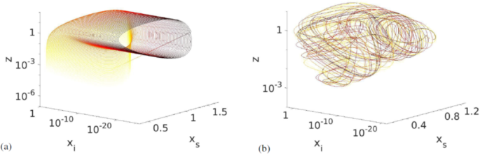
The evolution of the trajectories in xs − xi − z-space for different values of R. (a) at R = 1.025 where the system becomes quasiperiodic near the chaotic trasition. Other parameters were set to a = 7/400, b = 0.0208, c = 2, d = 0.3098. The fourth dimension, y, has been projected out. (b) Chaotic attractor for R = 1.5. The attractor has a characteristically streaked surface, and we estimate its dimension as D0 = 3.8 ± 0.1. The colour of the line indicates time, with darker colours signifying later times. Here, we have removed the initial transient.
Source: Ecology - nature.com
