Artificial light during the polar night disrupts Arctic fish and zooplankton behaviour down to 200 m depth

For each of the three experiments we used the RV Helmer Hanssen as our main research platform. During the experiments, the ship was drifting with the engine on but without any power on the propellers. Also, during all three experiments, the same level of noise, light field/intensity and activity were ensured in order to dismiss these factors as responsible for any difference in response between each experiment.

Species composition

At Station A, krill (Thysanoessa spp.) and capelin (Mallotus villosus) dominated the pelagic community, whereas Atlantic cod (Gadus morhua) and polar cod (Boreogadus saida) were the two most dominant taxa in the bottom trawl (Table 1). The Target Strength of these species have been shown to decrease when their tilt angle increases³⁹, for instance to dive away from surface illumination. The zooplankton community was dominated by copepods (mainly Calanus spp.) accounting for 98% of the community (total zooplankton abundance 22.7 (+/−6.9) ind. m⁻³). At Station B, northern shrimp (Pandalus borealis) and juvenile long rough dab plaice (Hippoglossoides platessoides) dominated in the bottom trawl while herring (Clupea harengus) and northern shrimp dominated the midwater trawl assemblage. Herring has been shown to react in a distinct way when exposed to artificial light, both as they pack in dense schools and by being attracted to artificial light⁴⁰. In contrast to krill and fish, change in the tilt angle of northern shrimp, for instance to avoid light at the surface, alter their target strength in a way that increases their acoustic target strength⁴¹. Zooplankton was abundant at Station B (73.4 (+/−10.6) ind. m⁻³) with the majority consisting of Calanus spp. (87%), krill (Thysanoessa inermis, 4%) and chaetognaths (Parasagitta elegans 5%). Trawling was not permitted at Station C, so at this location we do not have direct information regarding species composition of fish and larger macrozooplankton. Zooplankton net samples showed that the community consisted to 81% of copepods (Calanus spp., Metridia longa), as well as krill (5%) and chaetognaths (8%), but abundance was very low (1.6 (+/−0.6) ind. m⁻³).

Survey design

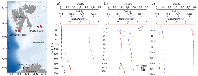
Artificial light experiments were conducted in situ from the RV Helmer Hanssen offshore the East coast of Spitsbergen (77°33.5’N 29°59.9’E) on 9 January, 2018, in Hornsund (76°56.3’N 16°15.8’E) on 14 January, 2018, and North of Tromsø (70°06.1’N 19°16.71’E) on 17 January, 2018 (Fig. 1, left panel). Lights used were normal working lights representative for any ship operating in the dark. All lights from the Helmer Hanssen were turned off for 49 min (9 January), 178 min (14 January) or 9 min (17 January) before being turned on again. Change in the acoustic backscatter was recorded from the hull-mounted EK60 echosounder (18, 38, and 120 kHz). The ping rate was set to maximum and pulse length to 1024 µs. The echosounder was calibrated using the standard sphere method⁴². A Seabird 911 Plus CTD® fitted with a Seapoint Turbidity sensor recorded temperature, conductivity and turbidity during each experiment.

To measure the spatial impact of artificial light footprint from the ship, an Acoustic Zooplankton and Fish Profiler (AZFP 38, 125, 200, 455 kHz; ASL Environmental Science, Victoria, Canada) was deployed from a small boat (Polarcirkel™) stationary, but at varying distances from the Helmer Hanssen. For the AZFP, we only analysed the data at 125 kHz because higher frequencies have a limited range and the 38 kHz dataset was corrupted by the hull of the Polarcirkel due to wide side lobes. Vertical resolution varied from 37 cm on 9 January, and 2 cm on 14 and 17 January. The pulse duration was 1000 µs, ping rate 0.33 Hz (i.e., 1 ping 3 s⁻¹) and source level was 210 dB (re 1 µPa at 1 m). The AZFP was calibrated by the manufacturer (± 1dB) prior to deployment. The AZFP and EK60 echosounder on the Helmer Hanssen were operated at the same stations, but not at the same time to avoid interferences.

Acoustic analyses

Acoustic data were scrutinised and cleaned with Echoview® 8. We used Echoview’s algorithms to remove background and impulse noise from EK60 and AZFP data, and attenuated noise signals from AZFP data^43,44. The echograms at 18, 38, 120 kHz (EK60) were divided in 1 min long x 3 m deep echo integration cells²⁵. The mean integrated Nautical Area Backscattering Coefficient (NASC in m² nmi⁻²) from the hull-mounted echosounder was compared with lights on and off for each station. We calculated the centre of mass of the backscatter to document changes in vertical distribution⁴⁵. For the AZFP, we stopped for 5 min near RV Helmer Hanssen, then at 50 m and afterwards every 100 m until 200 m (9 January), or 300 m (14 and 17 January). The centre of mass and total NASC at each stop were calculated at 125 kHz to assess the distance at which the lights from the ship impact the acoustic backscatter (i.e., proxies for the depth and biomass of scatterers).

Fish and zooplankton sampling

We deployed a Harstad pelagic trawl and a Campelen bottom trawl at stations A and B to groundtruth the acoustic signal. For safety reasons, the trawling was carried out with working lights turned on before the light experiments were initiated. All necessary licences and approvals were secured to carry out the trawling, which were always kept to an absolute minimum period. The Harstad trawl had an opening of 18.28 × 18.28 m and an effective height of 9–11 m and width of 10–12 m at three knots. The Campelen was trawled at three knots from 20 min and had an opening of 48–52 m, and a codend with an inner-liner mesh of 10 mm. All organisms were identified to species or genus onboard and we recorded the total number and weight of each species. Unfortunately, no trawl was deployed at Station C.

At Station A, we used a WP3 net (Hydrobios Kiel, 1 m² opening 1 mm mesh size) to take three zooplankton samples from 50 to 0 m. At stations B and C, zooplankton was sampled using a MIK net (Methot, Isaacs, Kidd Midwater Ring Net, 3.14 m² opening, 14 m long with main net bag of 1.5 mm mesh size, and the terminal 1.5 m part of 0.5 mm mesh size). Six vertical hauls were taken from 70 to 0 m at each station. All zooplankton sampling were conducted with working lights on the ship turned off. The samples were preserved in 4% hexamethylenetetramine-buffered seawater formaldehyde solution immediately after collection. In the laboratory, larger organisms (e.g., krill, chaetognaths, jellies) were identified and enumerated from subsamples using a plankton splitter (Station B) or from the entire sample (stations A and C). Copepods were counted from subsamples using a macropipette. Subsampling was continued until at least 300 individuals per sample were enumerated. Abundance estimates (individuals m⁻³) are based on filtered water volume measured by a flowmeter attach to the centre of the MIK net opening, and for the WP3 samples by multiplying mouth opening area of the net by vertical hauling distance assuming 100% filtration efficiency.

Light measurements

Absorption and light backscatter profiles were recorded at 9 wavebands across the visible spectrum using WETLabs AC-9 (light beam attenuation metre) and BB9 optical sensors, respectively. Data from both instruments were corrected for light absorption and scattering artefacts following standard manufacturer’s correction methods. The AC-9 was calibrated using freshly drawn Milli-Q ultrapure water on board the ship. Temperature and salinity corrections were applied using concurrent data from Seabird SBE19Plus CTD profiles. Irradiance from ship’s lights at the sea-surface was measured using a hyperspectral Trios RAMSES planar irradiance sensor, giving E_PAR = 2.24 μmol photons m⁻² s⁻¹ just beneath the surface. Retention of light (relative values) were measured from the open boat using a set of specially designed sensors to measure light in situ during the Polar Night²⁴.

The penetration of light at a given wavelength into the water column was calculated using the Beer-Lambert Law

where the diffuse attenuation coefficient, K_d(λ), was estimated from measurements of light absorption, a(λ), and backscattering, b_b(λ), using the relationship from⁴⁶

Here, the parameter g = 1.0395 and μ_d is the mean cosine for downwards irradiance and is estimated assuming light source at zenith (θ = 90°) and the relationship⁴⁷

Statistics and reproducibility

Statistical analyses (i.e., mean NASC) were conducted using RStudio Version 1.1.442. Echoview dataflow and Matlab code used for acoustic and light analyses, respectively, are available upon request.

Reporting summary

Further information on research design is available in the Nature Research Reporting Summary linked to this article.

Source: Ecology - nature.com