PLS description
Usefulness of PLS
Projections to latent structures (PLS), a more correct term for Partial Least Squares27, is a powerful multivariate method that is able to integrate data from different scientific disciplines in a single analysis22,24. It has minimum demands in terms of sample size, residual distribution and measurement scales28, while at the same time being able to handle a large amount of information on a relatively small number of independent observations. Allowing an analysis of crop performance that includes the many noisy and collinear variables related to farmers’ management choices as well as ecological, soil and landscape variables, the method is able to recognize farming systems and agro-ecosystems as complex social-ecological systems rather than simple bio-physical systems. Agro-ecosystems encompass ecological and decision networks and management inputs that are connected to one another and perform different functions leading to the provision of a wide range of ecosystem services, including crop yield and quality29.
Technical description
PLS is a partial least squares regression analysis and is used to find the relationships between two matrices X and Y22. It is a latent variable approach to modelling the covariance structures in these two spaces. While PLS is fairly well known in social sciences, marketing, psychology and education, it is also used for example in chemometrics24,27,30. One of the reasons for using PLS is the costs associated with including a large number of objects (individuals) in classical analyses. As an extension of Principal Component Analysis (PCA), PLS derives its usefulness from its ability to analyse data with many, noisy, collinear, and even incomplete variables in both X and Y. Details on the origins, evolutions and applications of PLS in the social sciences have been published previously, as well as the presentation of related methods in the family of multi-block analysis28,30,31. The performance of the PLS regression models improves with relevant X-variables that explain the most variation in Y variables. The PLS model diagnostic of its appropriateness, i.e. a model with optimal balance between fit and predictive ability32, is based on parameters R2Y (explained variation) and Q2Y (predictive ability). Details on the significance and evaluation of the goodness of fit (R2Y) and goodness of prediction (Q2Y) through the cross validation (CV) method under PLS have also been explained in a previous study and in other publications22,23,24. The goodness of fit and prediction of each response variable are obtained with PLS coefficients and the root mean square error (RMSE, %) is calculated to assess the predictive ability.
Farm choice and description
Thirty four farms were selected in two agro-ecological zones; the Swedish central eastern county (Uppsala County, around 60°N, 18°E) and the Swedish southern county (Scania County, around 55°N, 13°E). Due to latitude differences the two agro-ecological zones, hereafter called regions, differ in terms of climate that affects the growth and development of barley and soil processes. For both regions, seventeen farms growing spring barley (the most common annual crop) were selected including conventional farms and organic farms. Within organic farms, time since conversion to organic farming varied from 1 to 26 years, which enabled us to include a broad range of management practices as a result of management skills and experience developed over time. Three groups of farms were considered: conventional farms (CF), young organic farms (YOF) with less than 6 years since transition from conventional farming practices, and old organic farms (OOF) with 11 to 26 years since transition. Farms included mixed arable and livestock systems with cattle, pigs and/or horses in addition to pure arable farms. Sizes of the farms varied from 34 to 700 ha in Uppsala County and from 11 to 260 ha in Scania. The farms were selected to represent the length of the landscape complexity gradient in the regions. The distribution along the gradient went from complex landscapes with many non-crop habitats and forested areas to more homogenous agricultural landscapes with mainly arable land. Care was taken to select farms in such a way that all categories of farms (CF, YOF, OOF) were represented along the whole landscape gradient in each region33,34. The selected organic farms were certified by KRAV, the most common Swedish Trademark for organic products.
Survey of farm management practices
A questionnaire survey was conducted with the farmers in late 2011 and 2012 to obtain data on management practices on a given barley field for each farm in the present and recent past. Questions were directed to understanding the management at the whole farm level, with special focus on the management practices during the period 2009–2012 on one field per farm where barley was grown in 2012. Farm types, year of conversion to organic farming, and cultivar grown in 2012 were recorded (Table 1). All interviews were conducted on farm. The questions are provided in Table S1, along with the type of answers and corresponding management practices, which were considered for the analysis.
Due to the diversity of possible answers about management practices and resources used on farm, we aggregated them under a set of synthetic variables to reduce the number of independent variables in the analysis. In this way, we reduced the number of possible answers (variables) in the analysis from 132 to 29 variables, out of which 11 related to farm characteristics and 18 related to field management (Table 2). Aggregation procedures were detailed, for example for livestock density index, frequency of organic fertiliser application, etc., in a previous study23.
Barley performance indicators and weed cover
On each farm, one spring barley field was selected as a standard study crop, which is the second most important cereal in Europe35, for both humans and livestock. In Sweden, barley and winter wheat are the main cereal crops in terms of cultivated area with around 318 and 476 kha, respectively, in 201836. In 2017, the barley production was estimated at 447,900 tonnes in Scania and 145,800 tonnes in Uppsala county36. Spring barley was chosen as a model crop for its importance in terms of production but also because it is better distributed among different farm types; arable farms, mixed farms and specialised livestock farms. For each field, the landscape complexity around the field was determined according to the definition of landscape heterogeneity index33,34. In the case of more than one barley field on a given farm, a high landscape index (in the radius of 1 km) was the main criteria for choosing which barley field to study in order to increase the landscape complexity gradient when examining diversified management practices between conventional and organic farms. The LHI index is based on the proportions of semi-natural grassland and field border in the surroundings of the field23,37.
In 2012, seven barley performance indicators (BPIs) were measured in the selected spring barley field on each farm (see above). The BPIs included N concentration in the biomass (grain and whole biomass), and dry matter (DM) production at two growing stages: BBCH 31(stem elongation) and BBCH 87 (ripening: hard dough) according to Lancashire38. Biomass samples (4 random quadrats of 0.25 m2 per field, in total 1 m2) were cut at 5 cm above the ground and oven-dried at 60 °C for at least 24 hours. At harvest, BBCH 87, DM of straw and grain were separated. Samples were taken at a minimum of 20 meters from the edge of the field. Percentage weed cover was visually estimated during barley growth and an average percentage weed cover estimated on 18, 25 July and 2 August 2012 (for which data were complete for all the fields) was included as a variable affecting the BPIs beside the management practices. At the harvest, BBCH 87, the number of ears per sample was counted. Nitrogen concentration in the straw and grains was determined with an elemental LECO 2000CN analyzer.
Soil characteristics measurements
On each selected barley field, soil mineral N (SMN) was measured in on samples collected before fertilizer application early in the 2012 growing season (Table 2). In addition, total soil C and N (LECO 2000CN analyser), soil pH (1:2.5 H2O) and texture were measured in each selected barley field. The percentage of clay was used to represent the variation in soil texture.
PLS application
In this study, PLS was used to examine how different sets of explanatory variables (X) were related to the set of barley performance variables (Y) (see a schematic method description in Fig. 1). The X consisted of 28 management practices (aggregated from 100 variables originally measured), 5 soil and 1 landscape characteristics (X-matrix, 34 variables) and Y was barley performance indicators (Y-matrix, 7 variables). Variables influenced by regional location, e.g. because of climate differences, were standardized (e.g., sowing date, soil clay content). Each farm was considered as an object, a unit with complex interactions in the system. For farm level variables, obtained from the survey, one value was connected to each farm while at the field level the mean value of four samples were considered for both X and Y variables. Both PLS matrices can be expressed as: Y = TQ’ + F and X = TP’ + E, where matrix T contains X scores, the P matrix contains X loadings, matrix Q contains the Y loadings and F and E matrices are the residuals of the un-explained variation in Y and X tables. The relationship among the Y and X tables was derived through the latent variable T. The latent T variable represents the proportion of the explained interaction variance of the Y matrix by the set of variables from the X matrix. The number of T variables, or principal components (PC1 and PC2) in our figures, that are requested to optimally predict the dimensionality of the Y matrix, was determined by cross-validation procedure22.
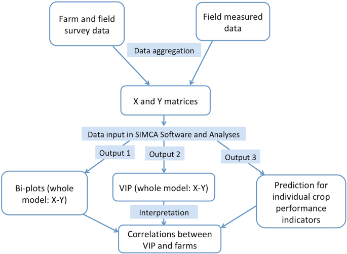
Schematic PLS method for on-farm data analysis linking socio-ecological factors and crop performance indicators. The analysis follows many steps and several combinations of variables to find the best model.
As the performance of the PLS regression models improves with relevant X-variables that explain the most variation of Y variables, we used the filter method with the variable importance in the projection (VIP) for variable selection39,40. This means that after the first model run including all the 34 X-variables, all variables with a VIP less than 1 were eliminated. A second model run with the remaining variables was done. Once the most valid model was reached, we obtained the model fit ability (cumulative R2Y, denoted R2Y (cum)) and the model predictive ability (cumulative Q2Y, denoted Q2Y (cum)) for all the dependent variables together and for individual dependent variables. Root mean square relative error (RMSE, %) was also calculated to measure the predictability of the PLS model. As the barley performance was measured with different indicators with different units and scales, the relative error is more meaningful than the absolute error. The RMSRE was calculated as
$${rm{RMSRE}}=100times sqrt{frac{1}{N}{sum }_{i=1}^{N}({frac{yi-widehat{yi}}{yi})}^{2}}$$
where yi is the observed value of the ith measured indicator, (widehat{yi}) is the corresponding PLS simulated value and N is the total number of fields.
A total of nineteen sets of X-matrices in relation to the barley performance (Y) were considered in the analyses. Three X-matrices (firstly, all the CF, YOF and OOF (Model 1: n = 34); secondly only YOF and OOF (Model 2: n = 22) and thirdly only CF (Model 3: n = 12)) were analysed and are fully presented as they fitted well with our study objective. The other 16 combinations of X-matrices were analysed to exclude the artefact that might be caused by the unbalanced contribution of different farm types. These included 6 matrices of 12 CF with 12 OF (Models 4–9, n = 24) and another 10 matrices with combinations of 6 OF from each region (Model 10–19, n = 12). The PLS analyses were performed with the software SIMCA-P V 13.0 (Umetrics, Umeå, Sweden).
Source: Ecology - nature.com

