In Jones et al. (2018) we describe a dataset uploaded to the Dryad Digital Repository (Dataset 112) comprising 63,070 unique raw time-lapse images captured by the Penguin Watch remote camera network, metadata for these photographs (e.g. date/time and temperature information), raw anonymised classifications from the Penguin Watch citizen science project, and ‘consensus clicks’ derived from these classifications10,13. Please refer to Jones et al. (2018 & 2019) for full details and an explanation of these data types.
Here we present a second dataset made available through the Dryad Digital Repository (Dataset 215). This contains two main file types. Firstly, files containing data directly derived from Penguin Watch citizen science classifications: Kraken Files and Narwhal Files (Online-only Table 2; produced using the Kraken Script and Narwhal Script, respectively), Narwhal Plots (Fig. 4 and Table 1; generated using the Narwhal Plotting Script), and Penguin Watch Narwhal Animations (Table 1, produced using GIMP (v2.8)21 and VirtualDub (v1.10.4)22. Secondly, files produced using computer vision – i.e. the Pengbot CNN (albeit initially trained on citizen science dot annotations): Pengbot Out Files, Pengbot Density Maps, and Pengbot Count Files (Table 2). All of these files directly relate to those provided in Dataset 112; i.e. an example within every file type is provided for each of the 63,070 raw time-lapse images captured by 14 cameras, meaning the processing pipeline can be traced for every photograph.
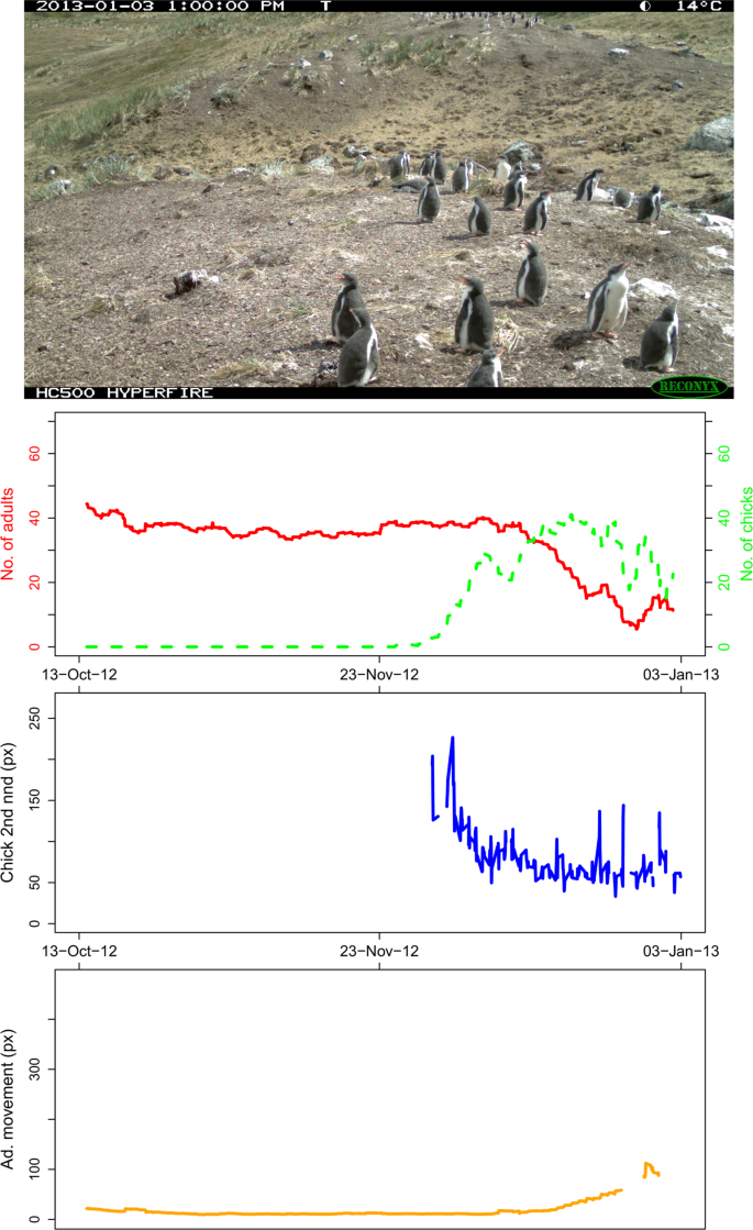
The Narwhal Plot for MAIVb2012a_000661 (the last image in the MAIVb2012a data set, therefore showing the complete trends for the data series). The plot comprises, from top down: the original time-lapse image (found in Dataset 112), graph 1: number of adults and chicks (moving average, n = 20), graph 2: average chick ‘second nearest neighbour distances’ (moving average, n = 2), and graph 3: mean adult ‘nearest neighbour distance’ between the ith and (i-1)th image (moving average, n = 20).
Also included in the repository (Dataset 215) are a Penguin Watch Manifest file, containing metadata for all of the images, and a Method Comparison File, which contains analysis of gold standard, citizen science and Pengbot counts for 1183 Penguin Watch images (see Technical Validation).
Explanation of terms
Citizen Science Workflow Files
Penguin Watch Manifest name:
Unique image reference for identification, in the format: SITExYEARx_imagenumber; e.g. DAMOa2014a_000001.
datetime: Time and date information for the image, in the format YYYY:MM:DD HH:MM:SS.
zooniverse_id: Unique identification code assigned to each image within Zooniverse (the online platform that hosts Penguin Watch – see www.zooniverse.org).
path: Folder pathway, which includes the image name (e.g. DAMOa/DAMOa2014a_000025).
classification_count: Number of volunteers who classified the image before it was retired.
state: State of completion – either complete (the image has been shown to the required number of volunteers) or incomplete (the image requires classification by further volunteers).
temperature_f: Temperature (in degrees Fahrenheit, as recorded by the camera) at the time the photograph was taken.
lunar_phase: Moon phase when the image was captured (one of eight options: “full” (full), “new” (new), “newcres” (new crescent), “firstq” (first quarter), “waxinggib” (waxing gibbous), “waninggib” (waning gibbous), “lastq” (last quarter) or “oldcres” (old crescent)).
URL: Link to an online thumbnail image of the time-lapse photograph (lower resolution than the raw time-lapse imagery included in the repository, but useful for reference).
Kraken Files
Kraken Files comprise filtered ‘consensus clicks’ and metadata (Online-only Table 2). The filtering threshold levels are ‘num_markings > 3’ for adults and ‘num_markings > 1’ for chicks and eggs (see Methods). Each row contains the following information. Please note that where ‘NA’ is given for probability values, ‘num_markings’, ‘x_centre’ and ‘y_centre’, no penguins have been identified in the image.
name: Unique image reference for identification, in the format: SITExYEARx_imagenumber; e.g. DAMOa2014a_000001.
probability_of_adult: Estimated probability that the corresponding individual is an adult – based on the number of volunteers classifying it as such, as a proportion of the total number of clicks on that individual.
probability_of_chick: Estimated probability that the corresponding individual is a chick – based on the number of volunteers classifying it as such, as a proportion of the total number of clicks on that individual.
probability_of_egg: Estimated probability that the corresponding marking indicates an egg – based on the number of volunteers classifying it as such, as a proportion of the total number of clicks on that area.
num_markings: The number of volunteer clicks that were aggregated to produce the ‘consensus click’ coordinate values (i.e. the number of individual clicks on a specific area of the image). Owing to the filtering process, num_markings is ‘>3’ for adults and ‘>1’ for chicks and eggs in the files provided alongside this Data Descriptor. These threshold levels can be changed in the Kraken Script, to create Kraken Files with different degrees of filtering.
x_centre: x coordinate value (in pixels) for the ‘consensus click’ (i.e. the coordinate calculated by the clustering algorithm)10,14. The origin (point 0, 0) is located in the top left-hand corner of the image, meaning it may be necessary to reverse the y-axis of a plot in order to overlay the ‘consensus clicks’ correctly. One coordinate value denotes one individual penguin/‘other’.
y_centre: y coordinate value (in pixels) for the ‘consensus click’ (i.e. the coordinate calculated by the clustering algorithm)10,14. The origin (point 0, 0) is located in the top left-hand corner of the image, meaning it may be necessary to reverse the y-axis of a plot in order to overlay the ‘consensus clicks’ correctly. One coordinate value denotes one individual penguin/‘other’.
For datetime, temperature_f, lunar_phase and URL please see ‘Penguin Watch Manifest’.
Narwhal Files
Narwhal Files contain penguin count data, ‘nearest neighbour distance’ metrics, and metadata. Each row contains the following information (Online-only Table 2):
imageid: Unique image reference for identification, in the format: SITExYEARx_imagenumber; e.g. DAMOa2014a_000001.
nadults: The total number of adults counted in the corresponding image, based on filtered (here, num_markings > 3) ‘consensus click’ data (see Kraken Files).
nchicks: The total number of chicks counted in the corresponding image, based on filtered (here, num_markings > 1) ‘consensus click’ data (see Kraken Files).
neggs: The total number of eggs counted in the corresponding image, based on filtered (here, num_markings > 1) ‘consensus click’ data (see Kraken Files).
adultndout: The mean adult ‘nearest neighbour distance’. Calculated by taking the distance between each adult and its nearest (adult) neighbour, and finding the mean average.
adultsdndout: Standard deviation of the adult ‘nearest neighbour distances’.
chickndout: The mean chick ‘nearest neighbour distance’. Calculated by taking the distance between each chick and its nearest (chick) neighbour, and finding the mean average.
chicksdndout: Standard deviation of the chick ‘nearest neighbour distances’.
chick2ndout: The mean distance between each chick and its second nearest (chick) neighbour within each image. The second nearest neighbour is calculated because the Pygoscelis penguins (the primary focus of the Penguin Watch camera network) usually lay two eggs. Since a chick’s nearest neighbour is therefore likely to be its sibling in the nest, the distance to the second nearest neighbour is calculated, to provide more information about the spatial distribution of chicks within the colony.
chicksd2ndout: Standard deviation of the chick ‘second nearest neighbour distances’.
meanchangeadult: Movement of each adult [j] between image [i-1] and image [i]. This is calculated by appending the xy coordinate of adult [j] in image [i] to a dataframe of the adult xy coordinates in image [i-1], and calculating the ‘nearest neighbour distance’ for adult [j]. The nearest adult to [j] is likely itself in the previous image, therefore this distance represents movement between the two images. It is possible that the nearest neighbour is a different individual, so a mean average is calculated to provide an indication of movement within the field of view. This metric is most appropriate between incubation and the end of the guard phase, when adults are often at the nest (see Methods).
meanchangechick: Movement of each chick [k] between image [i-1] and image [i]. This is calculated by appending the xy coordinate of chick [k] in image [i] to a dataframe of the chick xy coordinates in image [i-1], and calculating the ‘nearest neighbour distance’ for chick [k]. The nearest chick to [k] is likely itself in the previous image, therefore this distance represents movement between the two images. It is possible that the nearest neighbour is a different individual, so a mean average is calculated to provide an indication of movement within the field of view. This metric is most appropriate between incubation and the end of the guard phase, when chicks are at the nest (see Methods).
tempf: Temperature (in degrees Fahrenheit, as recorded by the camera) at the time the photograph was taken.
tempc: Temperature (in degrees Celsius) at the time the photograph was taken.
For datetime, lunar_phase and URL, please see ‘Penguin Watch Manifest’
Narwhal Plots and Penguin Watch Narwhal Animations
Narwhal Plots (see Fig. 4), generated using the Narwhal Plotting Script, provide a visualisation of summary statistics: graph 1: abundance of adults and chicks; graph 2: chick ‘second nearest neighbour distances’; and graph 3: mean adult ‘nearest neighbour distance’ between the ith and (i-1)th image. A plot is produced for each time-lapse image (Table 1), showing the moving average trends up to, and including, that image. Therefore, to see the complete trend, a plot should be created for the final image in the data series. The complete sets of graphs have been used to create Penguin Watch Narwhal Animations, which show the trends developing through time, alongside the time-lapse images. The folders of Narwhal Plots and Penguin Watch Narwhal Animations correspond to those described in Table 4 of Jones et al. (2018) (with the exception of PETEd2013, which is not included as it is a duplicate image set of PETEc2014).
Computer Vision (Pengbot) Files
Pengbot Out Files
Pengbot Out Files are MATLAB files containing a matrix of ‘penguin densities’, calculated using the Pengbot model. A density value is provided for each pixel in the corresponding raw time-lapse photograph. A file is provided (in Dataset 215) for each of the 63,070 images presented in Dataset 112; they are separated into folders according to camera (e.g. DAMOa_pengbot_out) (Table 2).
Pengbot Density Maps
A Pengbot Density Map (Dataset 215), generated using the Pengbot Counting Script (see Code Availability), is provided for each of the 63,070 raw time-lapse photographs presented in Dataset 112. The maps are a visual representation of the pixel densities presented in the Pengbot Out Files. Maps are stored in the database according to camera (e.g. DAMOa_density_map) (Table 2; Fig. 3, right).
Pengbot Count Files
These are generated using the Pengbot Counting Script (see Code Availability). They provide a penguin count (adults and chicks combined) for each image by summing the ‘penguin density’ of each pixel in the Pengbot Out Files (Table 2).
imageid: Unique image reference for identification, in the format: SITExYEARx_imagenumber; e.g. DAMOa2014a_000001.
raw_count: The number of penguins in the image, as calculated by the Pengbot model11. Since the counts are generated by summing pixel densities, they are unlikely to be an integer value.
count: The number of penguins in the image as calculated using Pengbot, rounded to the nearest integer.
Method comparison file
This file contains penguin counts for 1183 images, from four different cameras – DAMOa (Damoy Point; n = 300), HALFc (Half Moon Island; n = 283), LOCKb (Port Lockroy; n = 300) and PETEc (Petermann Island; n = 300) – as calculated by an expert (‘Gold Standard’), through Penguin Watch (‘Citizen Science’), and by Pengbot (‘Computer Vision’).
imageid: Unique image reference for identification, in the format: SITExYEARx_imagenumber; e.g. DAMOa2014a_000001.
datetime: Time and date information for the image, in the format YYYY:MM:DD HH:MM:SS.
GS_adults: The number of penguin adults in the corresponding image, as identified and calculated by an expert.
GS_combined: The number of penguin adults and chicks in the corresponding image, as identified and calculated by an expert.
CS_adults: The number of penguin adults in the corresponding image, generated using clustered citizen science data from the Penguin Watch project (threshold = num_markings > 3).
CS_combined: The number of penguin adults and chicks, as generated using clustered citizen science data from the Penguin Watch project (threshold = num_markings > 3 for adults and num_markings > 1 for chicks).
CV_rounded: The rounded number of penguin individuals (adults and chicks combined) in the corresponding image, calculated using the Pengbot model11.
The file also includes columns for six comparisons:
GS_combined vs. CV_rounded; GS_adults vs. CV_rounded; CS_combined vs. CV_rounded; CS_adults vs. CV_rounded; GS_combined vs. CS_combined; GS_adults vs. CS_adults.
Two columns are provided for each comparison. The first column shows the difference (in raw number of penguins) between the counts generated via the two methods. For example, if the gold standard combined count was 15 and the computer vision count was 12, then the ‘GS_combined vs. CV_rounded’ column would contain the value 3. The second column shows the same values, with any negative signs removed (whether the counts are under- or over-estimates is irrelevant when calculating average differences).
The average difference in counts, the standard deviation of this difference, the proportion of counts that are equal or differ by only one penguin, and the number of over- and under-estimates are also provided in the spreadsheet (and summarised in Table 3). Overestimates and underestimates relate to the second variable, i.e. for ‘GS_combined vs. CV_rounded’, an ‘underestimate’ would mean an underestimate by computer vision, as compared to the gold standard.
Source: Ecology - nature.com

