Sampling design
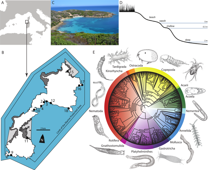
The Asinara National Park (http://www.parks.it/parco.nazionale.asinara/Eindex.php), located at the island of Asinara in the North-Western tip of Sardinia, Italy, covers a Marine Protected Area of about 110 km2. Before a National Park was established in 1997, the island hosted a hospital in the nineteenth century and then a prisoner camp and a maximum-security prison from 1885 to 1997 (ref. 38); nobody lives permanently on the island, and the only people who can impact marine biodiversity are tourists. The National Park receives an average of less than 1000 tourists every day during summer and almost no tourists from October to March; the total number of tourists is anyway limited, providing one of the best examples of potentially sustainable tourism along the coastline of the Mediterranean Sea3,38. Meiofauna on the island, even if disturbed by tourists, may have the possibility to recover during the tourist-free period from October to May. Asinara island is sinus shaped with four mountainous sections linked by a narrow, flat coastal belt (Fig. 1b). The tidal range in the area is just a few centimetres, making the physical impact of tides on meiofauna very limited. The west side of the island is rocky and steep, while the east side has flat areas occupied by coves and beaches. Most of the 11 beaches longer than 10 m are open to tourists, except for the two within the areas of total protection, corresponding to “Cala Sant’Andrea e Cala di Scombro di Dentro” at the centre and “Cala Arena e Punta dello Scorno” at the northern tip of the island (Fig. 1b).
We sampled all 11 beaches longer than 10 m present in the park (Fig. 1b). The beaches are mostly pocket beaches, between 20 m and 400 m along the shoreline, relatively homogeneous in their physical, ecological, and geographic conditions (Fig. 1d): they are within a maximum distance of 15.5 km, which minimizes spatial and biogeographic confounding factors; they are on the more protected Eastern coast of the island, which minimizes ecological factors of physical exposition to waves; and they are all sandy beaches, which minimizes ecological differences due to sediment granulometry. The major difference between the beaches is the number of tourists received during the summer months (Supplementary Data 1). The daily affluence of tourists ranged from beaches with no tourists to beaches with peaks of 300 tourists per day every 10 m2, even if such relatively high numbers were reached for only one or a few days in the season. Two major beaches (Cala Sant’Andrea and Cala d’Arena) within the areas of integral protection are restricted to the public (Supplementary Data 1). The number of tourists per beach was estimated by the authorities of the park by direct observations and the data are stored in their unpublished archives. The samples for the extraction of meiofauna were collected at the end of the tourist season between 22 September and 1 October 2014.
Sediment samples were collected manually. Each sample consisted of four replicates of 1 liter of sediments from the upper 5 cm of sand collected over a homogenous area of 1 m2 by scooping the top layer of sand with a jar. Immediately after collection, samples were taken to the laboratory on the island. All samples were processed within few hours after collection. Total meiofauna for metabarcoding with high-throughput sequencing (SI Appendix) was extracted from two replicates using the MgCl2 decantation technique15 through a mesh size of 63 µm and immediately preserved in ethanol at −20 °C. The other two replicates were used one for the analysis of sediment granulometry and one for morphological identification of meiofauna (see below).
Metabarcoding
Overall, 11 beaches were samples, with three levels (here called swash, shallow, and deep). Each of the 33 samples was sequenced twice for a total of 66 sequencing reactions; then, the replicate with the highest number of reads for each of the 33 samples was used for metabarcoding. Eight of the total 33 samples were discarded (Supplementary Data 1), due to the low quality of the DNA in both replicates. Sequence reads are publicly accessible at NCBI (GenBank) with accession number PRJNA369046. Index, adapter, and primers were removed with cutadapt 1.9.1 (ref. 39). The UPARSE pipeline was used for merging of sequences and quality control; USEARCH for the clustering of operational taxonomic units (OTUs)40,41. The pipeline was essentially used following the author’s online tutorial with the following settings: when merging sequences the maximum number of nucleotides that were allowed to be different in the overlap (max-diff) was set to 10 and the merged sequences had to have a minimum length of 300 bp. ZOTUs were calculated using the UNOISE algorithm, which attempts to identify all correct biological sequences in the reads (high-quality requirements and more than eight reads in the dataset) and cluster the other sequences around them, resulting in presumed 100% sequence identity termed ZOTUs for zero-radius OTU42,43. No rarefaction of the original raw data was performed in order to maintain all the sequences we obtained44; yet, we explicitly tested for the potential confounding effect of number of reads in the statistical tests (see below).
We used an iterative and phylogenetically informed approach for the taxonomic assignment of ZOTUs. Non-metazoan meiofaunal sequences, identified through Blast against the whole GenBank database, were discarded; meiofaunal metazoan sequences were assigned to the following 14 major taxonomic groups: Acari, Acoela, Annelida, Copepoda, Gastrotricha, Gnathostomulida, Kinorhyncha, Mollusca, Nematoda, Nemertea, Ostracoda, Platyhelminthes, Rotifera, and Tardigrada. Some of them, namely Acoela, Annelida, Gastrotricha, Gnathostomulida, Mollusca, Nemertea, Platyhelminthes, and Rotifera, are considered soft-bodied, are difficult to sample and preserve, and are often neglected in meiofaunal studies based on morphology18. Sequences were posteriorly assigned to each group using a neighbour joining tree including all recovered ZOTUs (Supplementary Fig. 1), aligned using a Q-ins-i refinement method implemented in MAFFT version 7 (ref. 45). Blast taxonomic assignments were then confirmed by building separated neighbour joining trees for each taxonomic group, adding all the overlapping sequences available in GenBank for each group at the date of March 2019 (Supplementary Figs. 2–20). Such additional analyses allowed us to be more confident about the taxonomic assignment of each ZOTU to each group at the desired taxonomic level (phylum, class, or order), regardless of the species or genus assignment, due to the potentially high number of unknown species in meiofauna18. Sequences were downloaded from GenBank, added to our dataset and handled for the analyses using the R packages rentrez 0.4.1 (ref. 46) and ape 3.2 (ref. 47). Only the ZOTUs that were eventually unambiguously nested within their target groups including identified GenBank sequences were retained, corresponding to the 99.9% of the metazoan sequences, and then the ZOTUs of non-strictly meiofaunal groups, e.g. Cnidaria, were removed (Supplementary Table 1).
Phylogenetic diversity was assessed from ultrametric trees obtained by BEAST package v2.4.8 (ref. 48) (Supplementary Figs. 21–26), using a Yule Process for tree priors and a generalized time-reversible (GTR) model for nucleotide evolution including a gamma distributed rate of variation among sites. Four chains run for 50 million generations, sampled every 10,000. Consensus trees were obtained after confirming convergence and discarding 10 million trees as burnin.
Morphological analyses
One of the four replicates collected for each sample was used to perform a parallel analysis on the effect of human frequentation on species identified using morphological criteria. These samples were processed mostly using the MgCl2 decantation technique but also by siphoning off the water just above the sediment, and using small variations in the methods, according to the focal taxon of study, as in previous studies covering different meiofaunal groups from the same samples18. Live material was studied using dissecting and compound light microscopes. Additional material for identification and/or descriptive purposes was preserved using methods appropriate for the respective taxon.
Due to the constraints in available taxonomic expertise and the long time that is needed to identify the whole species assemblages for each taxon, we focused on four main meiofaunal groups (Acoela, interstitial Annelida, Gastrotricha, and Platyhelminthes) only on six beaches (Supplementary Data 2). Identification of the specimens was performed using taxonomic keys and original literature according to the state-of-the-art systematics of each group.
Explanatory variables
As a proxy to account for the effect of human frequentation we used the maximum number of tourists for each 10 m2 of the analysed beaches, as measured by the records of the surveillance personnel of the park. Water depth was considered as a categorical explanatory variable (three fixed levels: 0 m, called swash; 0.3 m, called shallow; 2 m, called deep). Other potentially confounding factors that we included in our statistical models were: number of reads, intrinsic differences between beaches, and interactions between these factors, in addition to beach length and differences in sediment granulometry. Granulometry was assessed by passing 150 g of dry sediment through six sieves with mesh sizes corresponding to a range from 1 mm to 50 µm, shaking, fractioning, and weighing to obtain mean grain size, sorting coefficient, kurtosis, and skewness49,50 (Supplementary Data 1). From such measurements, we grouped sediments by granulometry by a k-means analysis to find the optimal number of groups, selected using Bayesian Information Criterion (BIC) for expectation–maximization algorithm initialized by hierarchical clustering for parameterized Gaussian mixture models51 using the mclust v5.3 R package52. All values were scaled before performing the analysis53. The highest BIC was obtained for 7 groups (BIC = −106.6, EEV ellipsoidal, equal volume, and equal shape multivariate mixture model). We accounted also for the effects of different length of each beach on the meiofaunal composition and richness by including such measure in the models.
Response variables
The effect of tourists was evaluated on three different types of community descriptors, included as response variables in the different sets of models: richness, community composition, and phylogenetic diversity. Richness was measured as the number of ZOTUs (or morphological species) for the total meiofauna and for each major group (defined as representing at least 5% of the total ZOTUs). Community differences between samples were measured using the Jaccard dissimilarity index from binary presence/absence data calculated with the R package betapart v. 1.5.1 (ref. 54). Phylogenetic diversity was measured as diversity and sorting at the phylogenetic level measured on ultrametric BEAST trees calculated only for the six taxonomic groups with more ZOTUs, in order to avoid biases due to low taxonomic diversity in the phylogenies. Phylogenetic diversity was calculated as Faith’s phylogenetic diversity (the sum of the total phylogenetic branch length for one or multiple samples) and as phylogenetic clustering (standardized effect size of the mean phylogenetic diversity (MPD), equivalent to 1-Nearest Relative Index, NRI55), with the R package picante 1.6-2 (ref. 56).
Statistical models
We developed statistical models to test the effect of tourists on meiofauna richness, community composition, and phylogenetic diversity. In order to mirror the complex structure of biological reality, our models included additional explanatory variables that could affect the response variables. To be able to account for a combination of such accounted and unaccounted effects in the models with richness and phylogenetic diversity as a response variable, we used GLMEMs, designed exactly for these kinds of analyses, with violations of the assumption that data are independent57. Thus, in the first set of GLMEMs we used number of tourists per 10 m2, depth (three levels: swash, shallow, deep), sediment granulometry (7 levels), and beach length, as explicit explanatory variables; the identity of the 11 beaches was included as a random effect to account for unmeasured differences between beaches and for spatial auto-correlation between samples within each beach. Then, we explored the effect of human presence separately for each depth using GLMs, including number of tourists per 10 m2, length of the beach, and type of sediment granulometry as explanatory variables. Before performing such detailed analyses, we assessed: (1) whether the assumption of differences between beaches and water depths held true, or rather they could depend on the confounding factor of number of reads by analysing their effect on each response variables using GLMs; (2) whether explanatory variables were correlated (they were not: absolute r values were below 0.52).
For GLMEMs and GLMs with ZOTU and morphological species richness as the response variable, we assumed a Poisson error structure in the models; for GLMs, we assumed a quasi-Poisson error structure when we found evidence of data over-dispersion. A Gaussian error structure was implemented for all models with phylogenetic diversity and phylogenetic sorting as the response variable. Model fit was checked for GLMs by plotting model residuals; plotting the predicted versus fitted residuals; using the normal Q–Q plot; checking Cook’s distances53. For GLMEMs, we checked the predicted versus fitted residuals. Results are presented always as Analysis of Deviance Tables from the R package car 2.1-3 (ref. 58). Analyses of Deviance Tables give a clear message on the effect of each variable, calculating the significance using likelihood ratio (LR) chi-square tests for GLMs and Wald (W) chi-square tests for GLMEMs58.
For models on community composition using matrices of Jaccard pairwise differences as a response variable, we assessed the percentage of the variability in community composition observed across samples using a permutational multivariate analysis of variance (PERMANOVA) in the R package vegan 2.2-1 (ref. 59). The structure of the models for community composition followed the same rationale of the analyses on ZOTU richness. All analyses were performed in R 3.6.3 (ref. 60).
DNA extraction and sequencing
DNA was extracted for metabarcoding from all 11 beaches. Each sample was vortexed for 10 s after which 6 ml were transferred to a small Petri dish and the ethanol was evaporated on a 60 °C hot plate on a sterile bench (approx. 2–5 h). An aliquot of 0.5 ml of extraction buffer (0.1 M Tris-HCl, 0.1 M NaCl, 0.1 M EDTA, 1% SDS, and 250 μg/ml proteinase K) was added to the dry sample, which was then incubated for 2 h at 56 °C. The sample was then re-suspended by vigorous pipetting and all the liquid was transferred to the micro-bead tube of the commercial PowerSoil extraction kit (MoBio). The kit was used according to the manufacturer’s protocol, except for the last step (elution of DNA from the spin column), for which twice 25 μl of elution buffer were incubated on the spin filter column for 15 min before centrifugation.
The primers used for Illumina sequencing were based on 18SF04 and 18SR22 (ref. 61). The selected primers amplify a DNA fragment of approximately 450 base pairs corresponding to the V1–V2 regions of the nuclear small subunit rRNA gene (18S rDNA). The coverage of the primer was, however, verified using the ARB software package62 with the SILVA reference database release 111 (ref. 63) and an ambiguous base was added to the reverse primer 18SR22: 5′-GCCTGCTGCCTTCCTTRGA-3′.
The DNA extracted from each sample was used as a template for amplicon library preparation, adopting a modified version of the Illumina Nextera protocol64. In particular, the library preparation was based on two amplification steps. In the first amplification, V1–V2 regions were amplified using the universal primers, reported above, having a 5′ end overhang sequence, corresponding to the Nextera Transposon Sequences (Illumina Adapter Sequences Document, Document # 1000000002694 v01 February 2016). Amplifications were performed using the Phusion High-Fidelity DNA polymerase system (Thermo Fisher Scientific). Each reaction mixture contained 0.5 ng of extracted DNA, 1× Buffer HF, 0.2 mM dNTPs, 0.5 μM of each primer, and 1 U of Phusion High-Fidelity DNA polymerase in a final volume of 50 μl. The cycling parameters for PCR were standardized as follows: initial denaturation 98 °C for 30 s, followed by 12 cycles of 98 °C for 10 s, 50 °C for 30 s, 72 °C for 15 s, and subsequently 18 cycles of 98 °C for 10 s, 62 °C for 30 s, 72 °C for 15 s, with a final extension step of 7 min at 72 °C65. All PCRs were performed in triplicate and in the presence of a negative control (Molecular Biology Grade Water, RNase/DNase-free water). The PCR products were visualized on a 1.2% agarose gel and purified using the AMPure XP Beads (Agencourt Bioscience Corp., Beverly, MA, USA), at a concentration of 1.2× vol/vol, according to the manufacturer’s instructions. The purified amplicons were used as templates in the second PCR round, which was performed with the Nextera indices priming sequences as required by the dual index approach reported in the Nextera DNA sample preparation guide (Illumina). The 50 µl reaction mixture was made up of the following reagents: template DNA (40 ng), 1× Buffer HF, dNTPs (0.1 mM), Nextera index primers (index 1 and 2), P5 and P7 primers at 0.2 µM and 1 U of Phusion DNA Polymerase. The cycling parameters were those suggested by the Illumina Nextera protocol. The dual indexed amplicons obtained were purified using AMPure XP Beads, at a concentration of 0.8× vol/vol checked for quality control on a 2100 Bioanalyzer (Agilent Technologies, Santa Clara, CA, USA) and quantified by the fluorometric method using the Quant-iTTM PicoGreen-dsDNA Assay Kit (Thermo Fisher Scientific, Waltham, MA, USA) on a NanoDrop 3300 (Thermo Fisher Scientific). Metagenomic libraries obtained were normalized to the 2 nM concentration, pooled, and sequenced on the MiSeq Illumina platform using the 2 × 300 paired-end (PE) approach. In order to increase the genetic diversity, as required by the MiSeq platform, a 5% of the phage PhiX genomic DNA library and a 40% of other genomic DNA libraries were added to the mix and co-sequenced.
Reporting summary
Further information on research design is available in the Nature Research Reporting Summary linked to this article.
Source: Ecology - nature.com
