Analysis workflow
This study was focused on the Canadian province of British Columbia, which covers 1 million km2, and has strong latitudinal, altitudinal, and longitudinal environmental gradients (from temperate rainforest to boreal forest, semi-desert, and dry grasslands). BC encompasses the most extensive undisturbed temperate rainforests, and some of the last free flowing rivers and intact vertebrate food webs in temperate North America. At the same time, much of the province has been under intense resource extraction pressure (timber, mining, natural gas) for nearly a century, and such extraction continues to contribute substantially to a growing domestic economy as well as foreign trade.
We used existing Life Cycle Assessment (LCA) studies to predict future GHG emissions for wind farms and run-of-river hydro, and combined combustion and upstream emission estimates for future projected natural gas development (e.g., shale gas extraction, processing, and transport). Second, we extracted the costs of electricity production ($/MWh) from both renewable sources, and from natural gas combustion from an existing dataset of all potential electricity sources, used in strategic energy planning in British Columbia38; we limited the dataset to potential development sites with electricity production costs of < $150/MWh to reflect current electricity markets39. Lastly, we estimated the spatial overlap of each energy technology with areas of high conservation priority in BC derived using systematic conservation planning principles40. We identified areas of high conservation value drawing on 385 vertebrate species distributions (341 small-bodied terrestrial species, 7 large-bodied carnivores and ungulates, and 37 fish species) and existing anthropogenic disturbance (i.e., forestry and linear infrastructure) under five prioritization scenarios: each of the three sets of species and anthropogenic disturbance separately, and a scenario combining all four datasets.
Energy datasets
To evaluate how potential energy development overlaps with areas of high conservation priority in BC we used a spatially-explicit dataset produced by the BC Provincial power utility BC Hydro (38; https://catalogue.data.gov.bc.ca/dataset/bc-hydro-resource-options-mapping-2013) that identified locations of potential electricity production (wind farms and run-of-river hydro) infrastructure38. Specifically, BC Hydro used topographic and climatic factors to identify the approximate sitting of individual renewable energy projects, as well as the spatial location of potential infrastructure associated with each project, such as access roads connecting each project to the nearest road network, and powerlines connecting each project to the provincial power grid38. While other energy technologies have been identified, wind farms and run-of-river hydro represent more than half of the potential renewable electricity generation in BC38, and nearly 8,000 potential development locations. We set a maximum development cost of $150/MWh to limit our analysis to a subset of economically viable projects, resulting in 66 run-of-river hydro locations and 87 wind farm locations (Fig. 1). We chose this threshold to be greater than the highest price paid for renewable energy in BC (up to $124/MWh in 2017) to allow for increases in the cost of electricity in the near future, but also to exclude sites that are cost-prohibitive in the near term. This threshold also reflects renewable electricity costs worldwide, which have been decreasing over the past two decades, and are forecast to decrease in the near term39. Energy cost estimates for wind and run-of-river locations are amortized for the lifetime of the projects (~30 years), include all infrastructure development (i.e., roads, power generation facilities, and powerlines), and are expressed in 2013 dollars38.
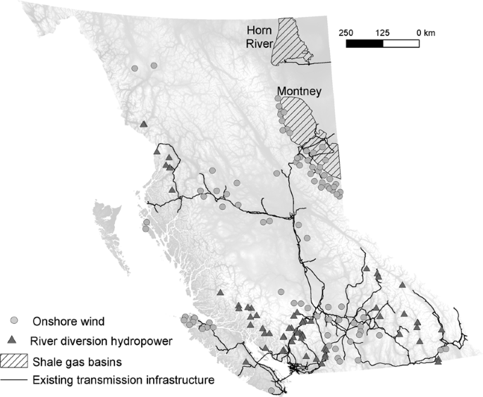
Spatial distribution of potential run-of-river hydro and wind farm facilities (projects < $150/MWh), and shale gas basins in British Columbia. Run-of-river hydro and wind farm data from BC Hydro Resource Options Report (2013); shale basins data from DataBC (https://apps.gov.bc.ca/pub/dwds/home.so). Maps produced using ArcGIS 10.5 (ESRI, Redlands CA, USA).
For each renewable energy technology, we considered the aggregate spatial footprint of run-of-river hydro and wind farm potential development locations along with their associated linear infrastructure. For wind farms, we built buffers around each point location of individual wind farms equal in area to the estimated footprint of that particular project (9.0–96.0 ha per facility). For run-of-river hydro, we built buffers around the project locations equal to the estimated footprint of the generating infrastructure (i.e., powerhouse, dam and headpond; 2.3 to 12.9 ha per facility). In addition to these project footprints, we used the estimated spatial location of powerlines, access roads and, in the case of run-of-river, the water pipelines (referred to as penstocks) connecting the dam to the powerhouse38, to evaluate the overlap of renewable energy development with conservation priorities (see section Evaluating overlap between energy development and conservation priorities).
For natural gas-generated electricity, we considered the footprint of natural gas extraction from shale, transport pipelines, and four proposed gas-fired power plants (with a range of the range of electricity costs dependent on the technology used, and size of the plant). However, these natural gas power plants have a small spatial footprint relative to the footprint associated with shale gas extraction. For natural gas extraction from shale, we considered the two major gas basins under exploitation in BC covering ~3.9 million ha (Fig. 1) (Horn River and Montney), as well as approved, but not yet developed, rights-of-way for gas extraction, refinement, and transportation infrastructure (roads, pipelines; www.data.gov.bc.ca/).
Life cycle assessment-based greenhouse gas emissions
We used GHG emission estimates from Life Cycle Assessment (LCA) expressed as grams of CO2 equivalent per kWh of energy produced for wind farms41, and run-of-river hydro42,43. LCA is a framework for evaluating environmental impacts of a project associated with all stages of its life, from extraction of raw materials, to manufacture, maintenance and disposal/recycling. For natural gas-generated electricity, we estimated GHG emissions by summing (1) estimates of the emissions generated from direct combustion38 with (2) estimates of upstream emissions (extraction, refinement, and transport of shale gas) produced using GHGenius 4.03 (www.ghgenius.ca). GHGenius is a peer-reviewed tool for estimating greenhouse gas emissions from a variety of fuels and industry sectors developed for Natural Resources Canada44. GHGenius is based on an existing Lifecycle Emissions Model45, and focuses on the lifecycle assessment of current and future fuels in transportation and electricity generation.
Biodiversity metrics
Small-bodied terrestrial vertebrates
We gathered occurrence locations for terrestrial vertebrate species from two open-access online databases: Global Biodiversity Information Facility (data.gbif.org) and Nature Counts (birdscanada.org/birdmon). We excluded species with fewer than 100 occurrence points within BC, which resulted in 341 native vertebrate species (15 amphibians and reptiles, 25 mammals, and 301 birds; Supporting Information S1) modeled using ensemble models46 implemented in program R47 via the biomod2 package48 (see Supporting Information S2).
Freshwater fish species
We used fish habitat suitability models for 37 species, including five native anadromous salmonids, Oncorhynchus spp. developed by the BC Ministry of Environment in support of the provincial Fisheries Sensitive Watersheds initiative (http://www.env.gov.bc.ca/wld/frpa/fsw/). These habitat models relate species occurrences in BC streams and rivers to stream and watershed physical attributes and ecological processes at the scale of subwatershed units (mean area = 4,920 ± 78 ha49).
Large-bodied carnivores and ungulates
We selected species that can be sensitive to broad-scale land-use development and that have well-documented range estimates. These constraints allowed us to consider to seven large mammals; bighorn sheep (Ovis canadensis), caribou (Rangifer tarandus caribou), elk (Cervus canadensis), fisher (Pekania pennanti), mountain goat (Oreamnos americanus), grizzly bear (Ursus arctos), and wolves (Canis lupus). Building on continental range estimates in previous work36, we refined each range map to British Columbia based on expert consultation within relevant government research bodies and the most recent status reports from the BC Ministry of Forests, Lands, and Natural Resources (bighorn sheep and elk50,51; fisher52; wolf53). These range maps were initially created as raster with 250 × 250 m cell size34, then rescaled to a 400 × 400 m resolution for use in the prioritization scenarios.
Existing landscape disturbance
Accounting for past landscape disturbance is critical for correctly identifying conservation priorities54. The province of BC has a relatively short (<100 years), but intensive history of landscape disturbance through resource extraction activities, including logging, mining, and oil and gas extraction. As a result, certain areas of the province have dense networks of infrastructure (roads, powerlines, pipelines, seismic lines), while other, less accessible and remote regions, are still relatively undisturbed by human activities. To account for legacies of past human disturbance, we used two landscape disturbance indicators summarized at the sub-watershed level (n = 19,469, mean area = 4,920 ± 78 ha), density of linear fragmentation (km/km2), and recent forest loss (1990–2012) from logging, wild fires, and pests (i.e., pine beetle). We used the Digital Road Atlas of British Columbia (http://geobc.gov.bc.ca/base-mapping/atlas/dra/), along with existing transmission and distribution lines38 to create a dataset of existing linear infrastructure in the province. We created a 100-m resolution layer of forest cover change between 1990 and 2012 by combining two spatial data sources: the 2013 Vegetation Resources Inventory (BC Ministry of Lands, Forests and Natural Resources Operations), a vector dataset of forest cover and logging activities in BC, and the Global Forest Change project55, a 30-m resolution global dataset of forest cover gains and loses derived from Landsat satellite imagery.
Overlap between energy development and conservation priorities
Identifying spatial conservation priorities
We used the systematic conservation planning methods and software Zonation v. 456 to identify top spatial conservation priorities in British Columbia under five scenarios that considered: (1) terrestrial vertebrate species (341 birds, amphibians, reptiles, and mammals [excluding large mammals]), (2) seven large mammal species, (3) 37 fish species, including the five species of anadromous salmon, (4) existing landscape disturbance from linear fragmentation (such as roads, pipelines, seismic lines, railroads) and recent forest loss (1990–2012, from logging, wildfires, and pests), and (5) a combination of the four previous species and landscape disturbance scenarios. Under the landscape disturbance scenario (scenario 4), conservation priorities were identified as areas that are intact (undisturbed habitat), as a proxy for intact species assemblages and food webs. For individual taxonomic group scenarios (1–4), each species was weighed equally within its own prioritization scenario. For the combined scenario, each of the four taxonomic and disturbance datasets were weighed equally; for example, each of the 341 terrestrial vertebrate species (dataset 1) were given a weight of 0.00294 (thus summing to 1), while each of the two disturbance layers in dataset 4 was given a weight of 0.5. This weighting system led to a balanced representation of the intact landscapes and the three different sets of species with different habitat and space requirements. When all four sets of data were combined, Zonation produced conservation prioritization outputs that maximized both biodiversity value (e.g., for each taxonomic dataset), and areas with the most undisturbed habitat.
Zonation produces a complementarity-based and balanced ranking of conservation priorities across the entire landscape57. Zonation calculates a rank order value of each cell in the landscape based on conservation priority (ranging from 0 = low conservation priority to 1 = high conservation priority). As a general rule, cells with rank values > 0.8 are considered to be of high conservation priority. Zonation is able to combine probabilistic species distributions data, large raster datasets (>108 grid elements), and can balance the distribution of species or communities with connectivity, costs, and needs of alternative land uses in the same prioritization58. For the purpose of this study, we used the additive-benefit function of Zonation with an exponent z = 0.25. Under this function, conservation value is additive across biodiversity features, and individual feature representation is converted via a benefit function that is in shape the same as the canonical species-area relationship (concave power function59). We also took into account existing protected areas, which cover ~10% of BC, using a hierarchical mask60. A hierarchical mask defines a strict sequence of cell removal, starting with the lowest values. In our case, the hierarchical mask was given a value of 1 for all protected areas, and 0 for the rest of the province. Thus, protected areas were given the highest conservation rank (top 10% of the province). The reasons for applying the hierarchical mask are twofold: (1) BC Hydro’s renewable energy planning process, as well as shale development, avoid existing protected areas, and (2) we aimed to focus our analyses on areas currently at risk from future energy development decisions. We excluded from the analyses all areas in the province covered by exposed rock, glaciers, barren lands, lakes, and urban areas. All the species, communities, ecosystems, and disturbance data were processed at a resolution of 400 × 400 m, with a resulting landscape of 5,131,698 cells with data.
Evaluating overlap between energy development and conservation priorities
Comparing the potential impacts of renewable and unconventional energy development poses several challenges. Foremost, our dataset on potential renewable energy development locations allowed us to calculate the length of new roads and powerlines, as well as the areal footprint of wind farm and run-of-river facilities, but there is no parallel dataset for future shale development. To evaluate the overlap between energy development and conservation priorities, we extracted the Zonation rank values for each cell intersected by the infrastructure of the 66 run-of-river hydro projects (n = 6,623 cells, of which 362 cells were buffer-based footprints, and the rest represented overlap with run-of-river linear infrastructure) and 87 wind farms (n = 13,383 cells, of which 1,240 cells were buffer-based footprints, and the rest represented overlap with wind farm linear infrastructure).
For shale development, we combined the locations of the two shale gas basins (Fig. 1) with the spatial footprint of approved, but not yet developed, rights-of-way for gas extraction, refinement, and transportation infrastructure outside the shale basins. Unconventional oil and gas extraction results in a network of well pads, access roads, pipelines, powerlines and seismic lines that tends to cover broad spatial areas61 compared to highly localized wind farms and run-of-river hydro and their estimated linear infrastructure. In addition, within the two BC shale gas basins, the exact footprint and location of future shale development is uncertain, and extraction activities are by nature, distributed across many individual wells. In the absence of exact locations of shale development infrastructure within the two shale basins, we randomly selected 10,000 points at which to extract ranks for each prioritization scenario and characterized the variation in Zonation ranks associated with current and future shale development. While this approach is different from the renewable energy footprint, the outcome (i.e., range of conservation ranks overlapped by energy infrastructure) is comparable, as we did not attempt to compare the three energy technologies in terms of their absolute footprint.
We quantified the overlap between potential energy development and conservation priorities produced from the Zonation outputs using probability density plots for the frequency of cells intersected by potential development across the range of Zonation ranks. A skewed distribution of Zonation ranks towards the highly-ranked cells (i.e., >0.7) is indicative of potential conflicts between conservation and energy development. For each energy technology, we calculated the proportion of cells corresponding to wind (13,383 cells), small hydro (6,623 cells) and shale development (10,000 cells) with conservation ranks > 0.7 under each prioritization scenario. Using density plots across the range of Zonation ranks instead of absolute measures of overlap (e.g., km2 impacted) allowed us to examine the relative overlap of potential shale development with conservation priorities without having to make assumptions about the future locations or density of shale infrastructure, and allowed a direct comparison with run-of-river hydro and wind farms.
We calculated the amount of renewable electricity that could be developed without impacting high conservation priority areas under each scenario (Zonation rank > 0.7, instead of >0.8, because protected areas accounted for the top 10% [0.9–1.0] of Zonation scores after applying the hierarchical mask60). While the overlap analysis evaluated trade-offs between the three energy sectors, this analysis provides complementary information, as it focuses on individual renewable energy projects by quantifying the potential energy gain from projects located in low conservation value areas. For each individual renewable energy project, we calculated the average and the range of Zonation ranks of cells intersected by its infrastructure (see above for description of infrastructure considered for potential renewable energy projects). We then ranked the 87 potential wind farms and 66 run-of-river hydro projects separately by their average Zonation rank value, and plotted the cumulative gain in annual electricity potential relative to the average and range of Zonation values.
Source: Ecology - nature.com

