Component response rate variation underlies the stability of highly complex finite systems

Component response rates of random complex systems

Complex systems (({bf{M}})) are built from two matrices, one modelling component interactions (({bf{A}})), and second modelling component response rates (γ). Both ({bf{A}}) and γ are square (Stimes S) matrices. Rows in ({bf{A}}) define how a given component (i) is affected by each component (j) in the system, including itself (where (i=j)). Off-diagonal elements of ({bf{A}}) are independent and identically distributed (i.i.d.), and diagonal elements are set to ({A}_{ii}=-,1) as in May¹. Diagonal elements of γ are positive, and off-diagonal elements are set to zero (i.e., ({boldsymbol{gamma }}) is a diagonal matrix with positive support). The distribution of diag(γ) over (S) components thereby models the distribution of component response rates. The dynamics of the entire system ({bf{M}}) can be defined as follows²⁰,

Equation 1 thereby serves as a null model to investigate how variation in component response rate (({sigma }_{gamma }^{2})) affects complex systems. In the absence of such variation (({sigma }_{gamma }^{2}=0)), γ is set to the identity matrix (diagonal elements all equal 1) and ({bf{M}}={bf{A}}). Under these conditions, eigenvalues of ({bf{M}}) are distributed uniformly¹⁵ in a circle centred at ((,-,1,0)) with a radius of (sigma sqrt{SC})¹ (Fig. 1a).

Effect of ({sigma }_{gamma }^{2}) on M (co)variation

The value of (Re ({lambda }_{max})), and therefore system stability, can be estimated from five properties of ({bf{M}})²¹. These properties include (1) system size ((S)), (2) mean self-regulation of components ((d)), (3) mean interaction strength between components ((mu )), (4) the variance of between component interaction strengths (hereafter ({sigma }_{M}^{2}), to distinguish from ({sigma }_{A}^{2}) and ({sigma }_{gamma }^{2})), and (5) the correlation of interaction strengths between components, ({M}_{ij}) and ({M}_{ji}) ((rho ))²². Positive ({sigma }_{gamma }^{2}) does not change (S), nor does it necessarily change (E[d]) or (E[mu ]). What ({sigma }_{gamma }^{2}) does change is the total variation in component interaction strengths (({sigma }_{M}^{2})), and (rho ). Introducing variation in (gamma ) increases the total variation in the system. Variation in the off-diagonal elements of ({bf{M}}) is described by the joint variation of two random variables,

Given (E[{gamma }_{i}]=1) and (E[{A}_{ij}]=0), Eq. 2 can be simplified,

The increase in ({sigma }_{M}^{2}) caused by ({sigma }_{gamma }^{2}) can be visualised from the eigenvalue spectra of A versus ({bf{M}}=gamma {bf{A}}) (Fig. 1). Given (d=0) and (C=1), the distribution of eigenvalues of A and M lie within a circle of a radius ({sigma }_{A}sqrt{S}) and ({sigma }_{M}sqrt{S}), respectively (Fig. 1a vs. 1b). If (dne 0), positive ({sigma }_{gamma }^{2}) changes the distribution of eigenvalues^23,24,25, potentially affecting stability (Fig. 1c vs. 1d).

Given ({sigma }_{gamma }^{2}=0), (Re ({lambda }_{max})) increases linearly with (rho ) such that²⁶,

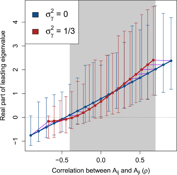
If (rho < 0), such as when ({bf{M}}) models a predator-prey system in which ({M}_{ij}) and ({M}_{ji}) have opposing signs, stability increases². If diagonal elements of γ vary independently, the magnitude of (rho ) is decreased because ({sigma }_{gamma }^{2}) increases the variance of ({M}_{ij}) without affecting the expected covariance between ({M}_{ij}) and ({M}_{ji}) (Fig. 2).

Figure 2

Complex system correlation versus stability with and without variation in component response rates. Each point represents 10000 replicate numerical simulations of a random complex system ({bf{M}}=gamma {bf{A}}) with a fixed correlation between off-diagonal elements ({A}_{ij}) and ({A}_{ji}) ((rho ), x-axis). Where real parts of eigenvalues of ({bf{M}}) are negative (y-axis), ({bf{M}}) is stable (black dotted line). Blue circles show systems in the absence of variation in component response rates (({sigma }_{gamma }^{2}=0)). Red squares show systems in which ({sigma }_{gamma }^{2}=1/3). Arrows show the range of real parts of leading eigenvalues observed. Because (gamma ) decreases the magnitude of (rho ), purple lines are included to link replicate simulations before (blue circles) and after (red squares) including (gamma ). The range of (rho ) values in which (gamma ) decreases the mean real part of the leading eigenvalue is indicated with grey shading. In all simulations, system size and connectance were set to (S=25) and (C=1), respectively. Off-diagonal elements of A were randomly sampled from ({A}_{ij}sim {mathscr{N}}{mathrm{(0,0.4}}^{2})), and diagonal elements were set to −1. Elements of (gamma ) were sampled, (gamma sim {mathscr{U}}mathrm{(0,2)}).

Full size image

Numerical simulations of random systems with and without ({sigma }_{gamma }^{2})

I used numerical simulations and eigenanalysis to test how variation in (gamma ) affects stability in random matrices with known properties, comparing the stability of A versus ({bf{M}}=gamma {bf{A}}). Values of (gamma ) were sampled from a uniform distribution where (gamma sim {mathcal{U}}(0,2)) and ({sigma }_{gamma }^{2}=1/3) (see Supplementary Information for other (gamma ) distributions, which gave similar results). In all simulations, diagonal elements were standardised to ensure that −d between individual (A) and (m) pairs were identical (also note that (E[{gamma }_{i}]=1)). First I focus on the effect of (gamma ) across values of (rho ), then for increasing system sizes ((S)) in random and structured networks. By increasing (S), the objective is to determine the effect of (gamma ) as system complexity increases toward the boundary at which stability is realistic for a finite system.

Simulation of random M across ρ

Numerical simulations revealed that ({sigma }_{gamma }^{2}) results in a nonlinear relationship between (rho ) and (Re ({lambda }_{max})), which can sometimes increase the stability of the system. Figure 2 shows a comparison of (Re ({lambda }_{max})) across (rho ) values for ({bf{A}}) (({sigma }_{gamma }^{2}=0)) versus M (({sigma }_{gamma }^{2}=1/3)) given (S=25), (C=1), and ({sigma }_{A}=0.4). For (-,0.4le rho le 0.7) (shaded region of Fig. 2), expected (Re ({lambda }_{max})) was lower in ({bf{M}}) than ({bf{A}}). For (rho ge -,0.1), the lower bound of the range of (Re ({lambda }_{max})) values also decreased given ({sigma }_{gamma }^{2}), resulting in negative (Re ({lambda }_{max})) in ({bf{M}}) for (rho =-,0.1) and (rho =0). Hence, across a wide range of system correlations, variation in the response rate of system components had a stabilising effect.

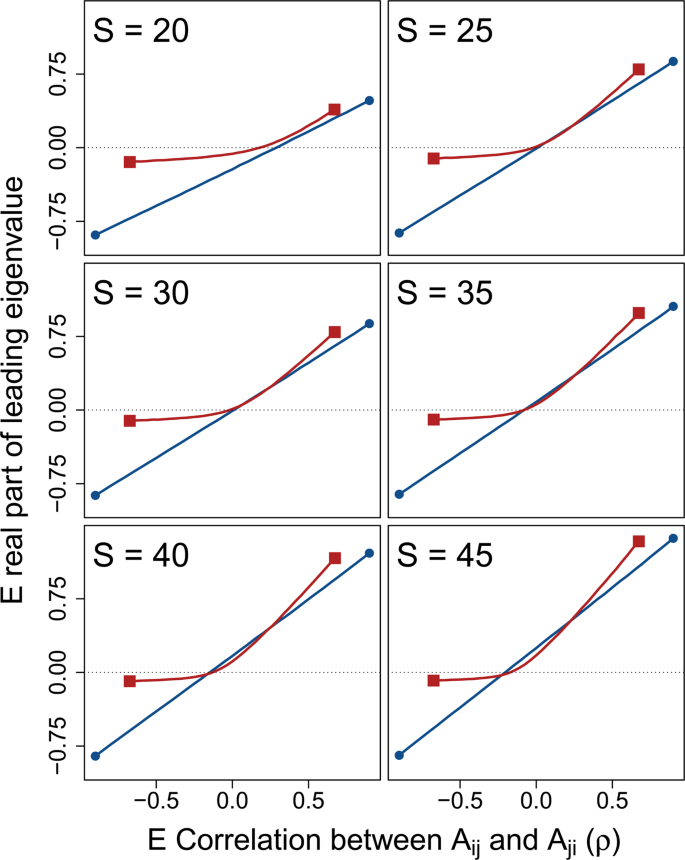
The stabilising effect of ({sigma }_{gamma }^{2}) across (rho ) increased with increasing (S). Figure 3 shows numerical simulations of ({bf{M}}) across increasing (S) given (C=1) and ({sigma }_{A}=0.2) (({sigma }_{A}) has been lowered here to better illustrate the effect of (S); note that now given (S=25), (1={sigma }_{A}sqrt{SC})). For relatively small systems ((Sle 25)), ({sigma }_{gamma }^{2}) never decreased the expected (Re ({lambda }_{max})). But as (S) increased, the curvilinear relationship between (rho ) and (Re ({lambda }_{max})) decreased expected (Re ({lambda }_{max})) for ({bf{M}}) given low magnitudes of (rho ). In turn, as (S) increased, and systems became more complex, ({sigma }_{gamma }^{2}) increased the proportion of numerical simulations that were observed to be stable (see below).

Figure 3

System correlation versus stability across different system sizes. In each panel, 10000 random complex systems ({bf{M}}=gamma {bf{A}}) are simulated for each correlation (rho ={,-,0.90,-,0.85,ldots ,0.85,0.90}) between off-diagonal elements ({A}_{ij}) and ({A}_{ji}). Lines show the expected real part of the leading eigenvalues of M (red squares; ({sigma }_{gamma }^{2}=1/3)) versus A (blue circles; ({sigma }_{gamma }^{2}=0)) across (rho ), where negative values (below the dotted black line) indicate system stability. Differences between lines thereby show the effect of component response rate variation ((gamma )) on system stability across system correlations and sizes ((S)). For all simulations, system connectance was (C=1). Off-diagonal elements of A were randomly sampled from ({A}_{ij}sim {mathscr{N}}(0,{0.2}^{2})), and diagonal elements were set to −1. Elements of (gamma ) were sampled such that (gamma sim {mathscr{U}}(0,2)), so ({sigma }_{gamma }^{2}=1/3).

Full size image

Simulation of random M across S

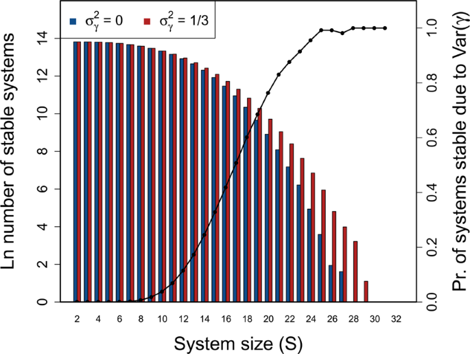
To investigate the effect of ({sigma }_{gamma }^{2}) on stability across systems of increasing complexity, I simulated random ({bf{M}}=gamma {bf{A}}) matrices at ({sigma }_{A}=0.4) and (C=1) across (S={2,3,ldots ,49,50}). One million ({bf{M}}) were simulated for each (S), and the stability of ({bf{A}}) vesus ({bf{M}}) was assessed given (gamma sim {mathcal{U}}(0,2)) (({sigma }_{gamma }^{2}=1/3)). For all (S > 10), I found that the number of stable random systems was higher in ({bf{M}}) than ({bf{A}}) (Fig. 4; see Supplementary Information for full table of results), and that the difference between the probabilities of observing a stable system increased with an increase in (S). In other words, the potential for ({sigma }_{gamma }^{2}) to affect stability increased with increasing system complexity and was most relevant for systems on the cusp of being too complex to be realistically stable. For the highest values of (S), nearly all systems that were stable given varying (gamma ) would not have been stable given (gamma =1).

Figure 4

Stability of large complex systems with and without variation in component response rate (γ). The log number of systems that are stable across different system sizes ((S={2,3,ldots ,49,50})) given (C=1), and the proportion of systems for which variation in (gamma ) is critical for system stability. For each (S), 1 million complex systems are randomly generated. Stability of each complex system is tested given variation in (gamma ) by randomly sampling (gamma sim {mathscr{U}}(0,2)). Stability given ({sigma }_{gamma }^{2} > 0) is then compared to stability in an otherwise identical system in which ({gamma }_{i}=E[{mathscr{U}}(0,2)]) for all components. Blue and red bars show the number of stable systems in the absence and presence of ({sigma }_{gamma }^{2}), respectively. The black line shows the proportion of systems that are stable when ({sigma }_{gamma }^{2} > 0), but would be unstable if ({sigma }_{gamma }^{2}=0) (i.e., the conditional probability that A is unstable given that M is stable).

Full size image

I also simulated 100000 ({bf{M}}) for three types of random networks that are typically interpreted as modelling three types of interspecific ecological interactions^2,27. These interaction types are competitive, mutualist, and predator-prey, as modelled by off-diagonal elements that are constrained to be negative, positive, or paired such that if ({A}_{ij} > 0) then ({A}_{ji} < 0), respectively² (but are otherwise identical to the purely random ({bf{A}})). As (S) increased, a higher number of stable ({bf{M}}) relative to ({bf{A}}) was observed for competitor and predator-prey, but not mutualist, systems. A higher number of stable systems was observed whenever (S > 12) and (S > 40) for competitive and predator-prey systems, respectively (note that (rho < 0) for predator-prey systems, making stability more likely overall). The stability of mutualist systems was never affected by ({sigma }_{gamma }^{2}).

The effect of ({sigma }_{gamma }^{2}) on stability did not change qualitatively across values of (C), ({sigma }_{A}), or for different distributions of (gamma ) (see Supporting Information).

Simulation of structured M across S

To investigate how ({sigma }_{gamma }^{2}) affects the stability of commonly observed network structures, I simulated one million ({bf{M}}=gamma {bf{A}}) for small-world¹⁶, scale-free¹⁷, and cascade food web^18,19 networks. In all of these networks, rules determining the presence or absence of an interaction between components (i) and (j) constrain the overall structure of the network. In small-world networks, interactions between components are constrained so that the expected degree of separation between any two components increases in proportion to ({rm{l}}{rm{o}}{rm{g}}(S))¹⁶. In scale-free networks, the distribution of the number of components with which a focal component interacts follows a power law; a few components have many interactions while most components have few interactions¹⁷. In cascade food webs, species are ranked and interactions are constrained such that a species (i) can only feed on (j) if the rank of (i > j).

Network structure did not strongly modulate the effect that ({sigma }_{gamma }^{2}) had on stability. For comparable magnitudes of complexity, structured networks still had a higher number of stable ({bf{M}}) than ({bf{A}}). For random networks, ({sigma }_{gamma }^{2}) increased stability given (S > 10) (({sigma }_{A}=0.4) and (C=1)), and therefore complexity ({sigma }_{A}sqrt{SC},gtrapprox ,1.26). This threshold of complexity, above which more ({bf{M}}) than ({bf{A}}) were stable, was comparable for small-world networks, and slightly lower for scale-free networks (note that algorithms for generating small-world and scale-free networks necessarily led to varying (C); see methods). Varying (gamma ) increased stability in cascade food webs for (S > 27), and therefore at a relatively low complexity magnitudes compared to random predator-prey networks ((S > 40)). Overall, network structure did not greatly change the effect that ({sigma }_{gamma }^{2}) had on increasing the upper bound of complexity within which stability might reasonably be observed.

System feasibility given ({sigma }_{gamma }^{2})

For complex systems in which individual system components represent the density of some tangible quantity, it is relevant to consider the feasibility of the system. Feasibility assumes that values of all components are positive at equilibrium^6,28,29. This is of particular interest for ecological communities because population density ((n)) cannot take negative values, meaning that ecological systems need to be feasible for stability to be biologically realistic²⁸. While my results are intended to be general to all complex systems, and not restricted to species networks, I have also performed a feasibility analysis on all matrices tested for stability. I emphasise that (gamma ) is not interpreted as population density in this analysis, but instead as a fundamental property of species life history such as expected generation time. Feasibility was unaffected by ({sigma }_{gamma }^{2}) and instead occurred with a fixed probability of ({mathrm{1/2}}^{S}), consistent with a recent proof by Serván et al.³⁰ (see Supplementary Information). Hence, for pure interacting species networks, variation in component response rate (i.e., species generation time) does not affect stability at biologically realistic species densities.

Targeted manipulation of γ

To further investigate the potential of ({sigma }_{gamma }^{2}) to be stabilising, I used a genetic algorithm. Genetic algorithms are heuristic tools that mimic evolution by natural selection, and are useful when the space of potential solutions (in this case, possible combinations of (gamma ) values leading to stability in a complex system) is too large to search exhaustively³¹. Generations of selection on (gamma ) value combinations to minimise (Re ({lambda }_{max})) demonstrated the potential for ({sigma }_{gamma }^{2}) to increase system stability. Across (S={2,3,ldots ,39,40}), sets of (gamma ) values were found that resulted in stable systems with probabilities that were up to four orders of magnitude higher than when (gamma =1) (see Supplementary Information), meaning that stability could often be achieved by manipulating (S) (gamma ) values rather than (Stimes S) ({bf{M}}) elements (i.e., by manipulating component response rates rather than interactions between components).

Source: Ecology - nature.com