The stability of mutualism

The random matrix model

The present work is built around a variation of Robert May’s¹⁸ analysis introduced in the 1970’s to study the controversial question: “Will a large complex system be stable?” Instead of May’s linear dynamics, the classical nonlinear Lotka–Volterra equations of multi-species systems are taken advantage of. For a community of n-species, the Lotka–Volterra equations posit that the rate of change of the i’th species can be modelled by the nonlinear differential equations:

Here N_i is taken to be the population density of species-i. The interaction coefficients are described in the matrix A = (a_ij), where the element a_ij represents the effect species-j has on the growth of species-i. A is treated as a random matrix with interactions a_ij assigned randomly having zero mean and standard deviation σ, unless otherwise stated. A cooperative or mutualistic (+/+) interaction implies both a_ij > 0 and a_ji > 0, while a competitive (−/−) interaction is just the opposite. Exploitative interactions are of the form (+/−).

Intraspecific interactions a_ii are scaled to unity such that a_ii = −1. Following many other studies^{21,28,29,30,31,32,33,34}, to help gain analytical insights into the model’s properties, the growth rates are all given the scaling r_i = +1, an assumption that is also relaxed in what follows (see Supplementary Notes 3). But in the context of mutualistic communities, a positive growth rate reflects a property of facultative mutualism for species that have the capability of surviving on other resources in the absence of their mutualist partners^1,32,33. The advantages and disadvantages of this approach are discussed in the “Methods” section.

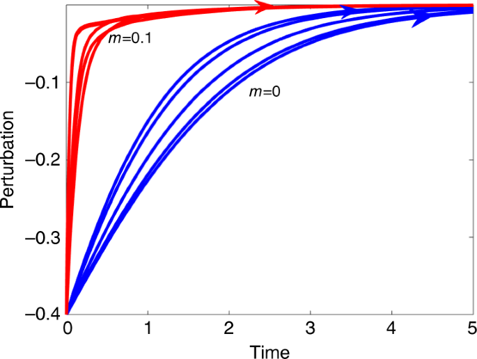
Before proceeding to the theoretical analysis, it is an appropriate point to introduce directly one of the key phenomena to be investigated. Figure 1 plots trajectories of a perturbed n = 10 species Lotka–Volterra model (Eq. (1)) as it returns to equilibrium. The perturbation mimics a species that has been considerably depressed in population numbers over a short time period (sometimes referred to in the ecological literature as a “pulse perturbation”^27,35). The pulse pushes the system out of equilibrium. One set of simulations (blue lines) has random interaction coefficients with mean strength (m = E(a_{{mathrm{ij}}}) = 0.0) and (sigma = 0.05) indicating each interaction is equally positive or negative. The second set of simulations (red lines) are of purely mutualistic systems having random interactions with mean (m = E(a_{{mathrm{ij}}}) = 0.1) and (sigma = 0.05), so that all interspecific interactions are positive ((a_{{mathrm{ij}}}, > , 0)) and mutualistic.

Fig. 1: Resilience of Mutualism.

Trajectories of a perturbed n = 10 species Lotka–Volterra model Eq. (1) as it returns to equilibrium. Blue lines are systems with random positive and negative interaction coefficients having (m = E(a_{{mathrm{ij}}}) = 0.0,,{mathrm{and}},,sigma = 0.05). Red lines are simulations mutualistic systems having random interactions with (m = E(a_{{mathrm{ij}}}) = 0.1), (sigma = 0.05) and all interactions positive. For all simulations, the population is depressed by 0.4 units initially, and the perturbation dies in time to zero. It is easy to see that the return time is much faster for the mutualistic systems. Note that five independent simulations are plotted for each value of (m) with identical initial conditions. Supplementary Fig. 1 in Supplementary Notes 2 similarly explores the effects of perturbing some 20 species when there are n = 100 species in total.

Full size image

An established and well recognized method for assessing the “degree of stability” of an ecological community requires measuring and comparing the recovery times from such a perturbation^15,27,36. [The method was employed by May¹⁵ specifically for mutualist models since at least the 80’s.] From Fig. 1, it is immediately clear that for the perturbed species of the purely mutualistic community (red lines), the return time to equilibrium, is far more rapid indicating far higher resilience. (To assist comparisons, species equilibrium levels have all been translated to appear as zero on the y-axis i.e., representing a perturbation of zero.) This much faster recovery time for mutualistic communities stands in contrast to the consensus view which characterizes mutualism as destabilizing, and is counterintuitive to much of what may be encountered in the theoretical ecology literature. But interestingly, a search through the literature reveals that Addicott³² had noted the possibility that mutualists have faster recovery time in simulations runs, but this was never explained or explored further by theoretical means. In short then, how can we make sense of this unusual resilience property of mutualistic communities, and is it a characteristic or a pathological occurrence?

Degree of stability and resilience

Let us analyse model system (1) in further depth. By setting all time derivatives to zero, it is possible to solve for the equilibrium populations (N_{mathrm{i}} = N_{mathrm{i}}^ ast) The equilibrium is deemed “feasible” if all equilibrium populations are positive ((N_{mathrm{i}}^ ast, > , 0)), which is an essential criterion for a viable ecosystem. As noted by Roberts²⁹, an unusual feature of this model is that feasible equilibria are nearly always locally stable and will return to equilibrium after a small perturbation, at least for the reasonable scaling of parameters chosen (see also Stone³⁷). A full stability analysis requires studying the n eigenvalues (lambda _i) of the community matrix S = DA, where ({mathbf{D}} = {mathrm{diag}}(N_1^ ast ,N_2^ ast , ldots .,N_{mathrm{n}}^ ast )) is a diagonal matrix. This is the major difference of the work presented here and the mainstream random matrix methods of Allesina and Tang²⁵, who study the eigenvalues of A rather than the community matrix S.

Following convention, we refer to Λ as the largest eigenvalue of the community matrix S = DA i.e., (Lambda = max _{mathrm{i}}left{lambda _{mathrm{i}}right}). (If the eigenvalues are complex we set (Lambda = max _{mathrm{i}}Releft{ {lambda _{mathrm{i}}} right})). When Λ < 0 the system is locally stable and will return to equilibrium after a small perturbation. However, if Λ > 0, the system is unstable. The degree of the system’s stability or resilience may be quantified by the magnitude |Λ|, which is an index of the system’s return time to equilibrium after a small perturbation³⁶. This is based on the knowledge that the eigenvalue associated with Λ is characteristic to the trajectory’s slowest eigendirection on its return to equilibrium. It is therefore considered the bottleneck. The more negative is Λ (the larger is |Λ|), the faster the trajectory can return to equilibrium, and the “more stable” and the more resilient is the system. In summary, when the system is perturbed from a feasible equilibrium by a small perturbation, the “slow dynamics” as the trajectory converges back to equilibrium is controlled by the largest (least negative) eigenvalue Λ and its associated eigenvector.

We will be making use of the Chen and Cohen scheme (see “Methods” section) which generates specially designed interaction matrices A in which the proportion of each interaction type is specified in advance. (For example, P = 75% mutualists, 15% exploitative and 10% competitive; see also ref. ²⁰). Several studies have examined the critical eigenvalue stability index Λ as the proportion P of mutualistic interactions is increased. In practice, for each P, this requires randomly choosing a proportion P of the n(n − 1) off-diagonal interactions elements ((a_{{mathrm{ij}}})) and assigning them to be of type (+/+), while the remainder (1 − P) are set to be exploitative (+/−), as explained in the “Methods” section. It was also possible to allow for the network’s connectivity C which simply ensures there is a fixed proportion C of non-zero interactions.

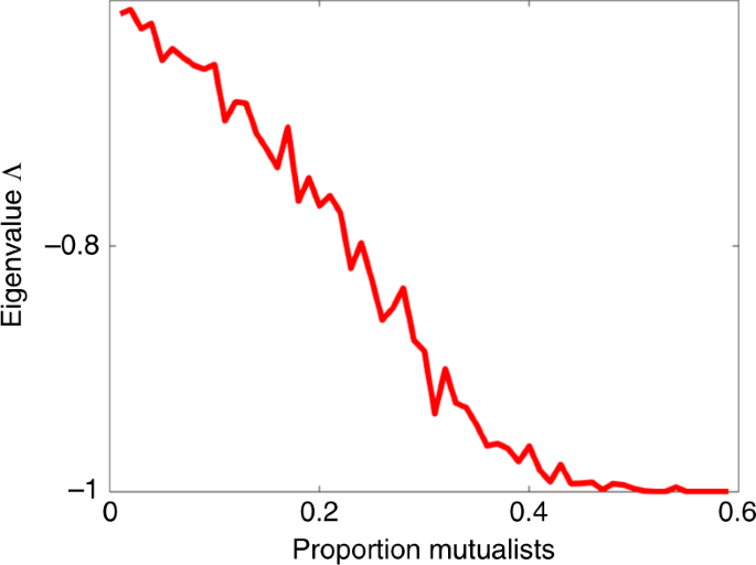
Figure 2 shows that resilience increases, with Λ becoming more negative as the proportion P of mutualistic interactions increases, until a saturation point at ({mathrm{Lambda }} = – 1) is reached. In these simulations, all community interactions were taken to be random with an exploitative structure, while mutualistic interactions were externally introduced to the proportion P required. But the results were qualitatively unchanged if the background interactions were competitive or purely random.

Fig. 2: The critical stability eigenvalue (Lambda).

The eigenvalue Λ is plotted as a function of P, the proportion of mutualistic interaction pairs, as an average of 50 runs. The more negative is Λ, the more stable is the (feasible) system in the sense that it has faster return time to equilibrium³⁶ and thus higher resilience. Parameters: n = 100 species; interaction variability σ = 0.02; connectance C = 0.7; growth rates (r_{mathrm{i}} = 1).

Full size image

The relationship is not difficult to explain. As will be shown, in large complex systems as Eq. (1), an increase in the proportion of mutualistic interactions P helps build up the equilibrium densities of individual species. For these feasible systems, higher equilibrium numbers translate into stronger stability, similar to a “stability in numbers” effect This link between high equilibrium numbers and strong stability has been demonstrated previously^22,37. In the context, of feasible competition communities where interactions strengths can reach relatively high levels it has been shown³⁷ that (lambda _{mathrm{i}} cong – ( {1 + E( {a_{{mathrm{ij}}}} )} )N_{mathrm{i}}^ ast). This appears to be different to the result in ref. ²² and a derivation is given in Supplementary Notes 1 together with assumptions (e.g., that growth rates (r_{mathrm{i}}) = 1, and perturbations of interactions are relatively small as discussed extensively in ref. ³⁷).

Feasible mutualist systems have relatively weak interactions, and thus in practice the critical eigenvalue component ({mathrm{Lambda }}) can be well approximated by the minimum equilibrium population (N_{{mathrm{min}}}^ ast), through the relationship:

(The latter formula takes into account that the stability matrix S always has an outlier eigenvalue λ_i = −1 as explained in the “Methods” section.)

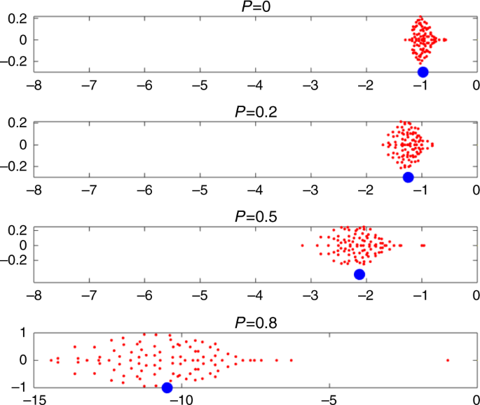
To explore this further, in Fig. 3 the eigenvalues of the community matrix S = DA are plotted for systems of n = 100 species and for P = 0, 0.2, 0.5, and 0.8. Each subplot gives an elliptical distribution for its 100 eigenvalues (lambda _{mathrm{i}}) in the complex plane (red dots), as predicted by random matrix theory²⁵. Adding cooperative interactions (i.e., increasing P), pushes the ellipse to the left. The center of the ellipse can be well approximated by the mean equilibrium population level (- N_{mathrm{i}}^ ast) plotted as a blue filled circle, indicating how the equilibrium populations increase in tandem with the eigenvalue distribution (see “Methods” section, Eq. (3)).

Fig. 3: Eigenvalue distributions.

Eigenvalues (lambda _{mathrm{i}}) of the Jacobian or community matrix in the complex plane, for four different values of P. Imaginary parts Im(λ_i) versus real parts Re(λ_i) are plotted. The “bulk” eigenvalues (red dots) are contained in an ellipse which centers close to the mean equilibrium level, i.e., (- N_{mathrm{i}}^ ast) plotted as blue circles. Stability becomes stronger (ellipse shifts to the left) as the proportion P of mutualistic interactions increases in otherwise exploitative communities. When P > 0.4, the largest outlier eigenvalue is (Lambda = – 1) (see Eq. (2)). For P = 0.8, it was necessary to stretch the scale for the x-axis and it is different to the other panels. Parameters: n = 100 species; interaction variability σ = 0.02; connectance C = 0.7; growth rates (r_{mathrm{i}} = 1), as in Fig. 2.

Full size image

A closer examination of the eigenvalue distribution reveals a well known formation in random matrix theory, namely that a multitude of “bulk” eigenvalues are located in the ellipse, while there is an additional “outlier” eigenvalue ({mathrm{Lambda }} = – 1), most easily noticeable for (P ge 0.4).

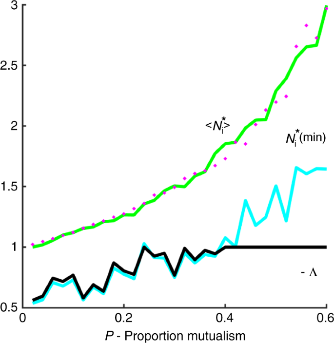
Figure 4 demonstrates that Eq. (2) does indeed hold. For each value of P, the equilibrium value of the species with the minimum population is plotted in red. As predicted, the minimum equilibrium value (N_{{mathrm{min}}}^ ast) of the populations (red line) is a good approximation to the critical eigenvalue −Λ (black line) in the regime (N_{{mathrm{min}}}^ ast, <, 1) (where P < 0.42). Outside of this regime, for higher values of P, the critical eigenvalue is then Λ = −1.

Fig. 4: Equilibrium populations.

The critical eigenvalue (Lambda) (black line) is plotted as a function of P, the proportion of mutualists. The minimum equilibrium value (- N_{{mathrm{min}}}^ ast) of the populations (blue line) is a good approximation to the critical eigenvalue (Lambda) in the regime (N_{{mathrm{min}}}^ ast, <, 1). Outside of this regime (Lambda = – 1). Plotted in green is (langle N_{mathrm{i}}^ ast rangle) which should be a proxy for the magnitude of the bulk eigenvalues (Eq. (3)). The magenta circles plot the approximation (N_{mathrm{i}}^ ast) ≃ (1/[1 – left( {n – 1} right)mCP]). Parameters, as in Figs. 2 and 3: (n = 100) species, (sigma = 0.02), C = 0.7; growth rates (r_{mathrm{i}} = 1).

Full size image

Bulk eigenvalues and short-term recovery

Until now we have examined the system’s return time, and thus resilience, but based on the assumption that the initial perturbation from equilibrium is very small. For larger perturbations, the short term recovery of disturbed populations is controlled by the “bulk eigenvalues” of the stability matrix. To see this, consider Fig. 3 where it is clear that as the proportion P of mutualistic interactions increases, the cluster of (n − 1) “bulk eigenvalues” associated with the random matrix “moves to the left” and separates out more and more from the “outlier” eigenvalue (lambda = – 1). It is interesting to examine how this affects the dynamics of the ecological system. To do so, we will assume that the population of a single species is depressed to a low abundance level by a pulse perturbation^27,35, as in Fig. 1. The resulting transient dynamics of the population trajectory then roughly passes through two distinct recovery phases.

Phase 1: The rapid first phase response is controlled by the large magnitude “bulk” eigenvalues (rather than the outlier (lambda = – 1)) which ensure rapid population growth and recovery. These eigenvalues generate the “fast dynamics” and ensure the model’s trajectory rapidly reorients itself towards the direction of the single positive equilibrium vector ({boldsymbol{N}}^{mathbf{ ast }}) (itself an eigenvector). As this swiftly takes place, the trajectory in any case ends up very close to equilibrium, as seen in Fig. 1. This first phase describes, what was referred to by Arnoldi et al., as the “short term recovery” phase²⁷.

Phase 2: Once in the vicinity of the equilibrium, the trajectory is then mostly controlled by the the smallest magnitude outlier eigenvalue, usually (lambda = – 1). It then “crawls” at a less rapid pace (along the associated eigenvector) as it converges to the equilibrium ({boldsymbol{N}} = {boldsymbol{N}}^{mathbf{ ast }}) at a rate determined by the eigenvalue (lambda = – 1), again seen in Fig. 1. This phase describes the longer term recovery time.

Interestingly Phase 2 is traditionally used to measure the return time to equilibrium and the resilience, because, as mentioned, it is perceived as the bottleneck. However, in many cases, as in the context here, it is Phase 1 which is the more relevant measure of recovery and resilience. This is because at the end of Phase 1, the trajectory has almost reached equilibrium, and any remaining discrepancy is in practice negligible.

Thus, with regard to resilience, the critical eigenvalue ({mathrm{Lambda }}) is only the part of the story and represents the speed at which the system returns to equilibrium in the single slow direction of a single key eigenvector. Figure 3 allows us to see that when the proportion P of mutualists increases, all the other “bulk” eigenvalues become substantially more negative. The elliptical distribution of the bulk eigenvalues is centered on the average equilibrium population level (- N_{mathrm{i}}^ ast) marked as a blue circle, whose magnitude increases greatly with P. Thus the speed to equilibrium from all other (n − 1) eigenvector directions increases substantially with higher levels of inter-species cooperation P. The short term recovery is thereby controlled by the high magnitude bulk eigenvalues, and is more rapid for larger P values.

An easy argument makes it possible to explain why mutualistic interactions tend to increase species equilibrium values (N_{mathrm{i}}^ ast) in this model. As discussed in Stone^37,38, the underlying “uniform model” (in which all interspecies interaction coefficients (a_{{mathrm{ij}}} = m) and (sigma ^2 = {mathrm{Var}}(a_{{mathrm{ij}}}) = 0.0)) acts as a skeleton framework and should be viewed as a good zero’th order approximation when perturbations are small. For the uniform model ((sigma = 0)), the mean equilibrium value is (N_{mathrm{i}}^ ast = 1/[1 – left( {n – 1} right)mCP]), where P is the proportion of mutualistic interactions and C is the connectance (see Supplementary Notes 1). The RHS of the equation is plotted in Fig. 4 (magenta circles) and provides a close fit to the mean value of the random matrix populations when (sigma, > , 0). This shows us directly why mutualism (in terms of P) builds up the equilibrium populations in the Lotka–Volterra model.

It is also important to note that going beyond a threshold of too many mutualistic interactions can lead to population blowup and loss of feasibility. To see this in simple terms, suppose all interactions are mutualistic of strength (a_{{mathrm{ij}}} = + m, > , 0). The assumption leads us to the “regular” model in which all species are identical. The model Eq. (1) at equilibrium yield: (N^ ast = 1/[1 – left( {n – 1} right)m]) for the case where C = P = 1 (see Supplementary Notes 1). Clearly, we must have the limitation (m, <, 1/left( {n – 1} right)) to prevent blow-up, and feasibility is lost if there is equality (see refs. ^37,38). These are important factors that constrain the feasibility of mutualistic systems.

Source: Ecology - nature.com