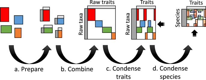
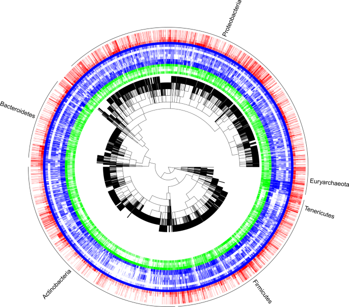
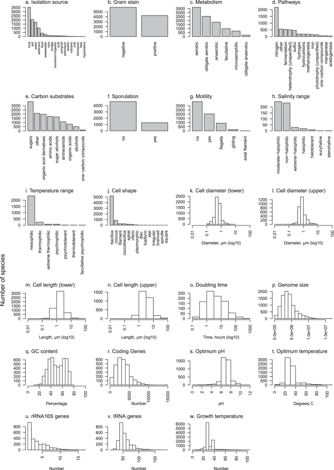
The scripted workflow was developed to reproducibly (a) prepare datasets to be merged; (b) combine datasets; (c) condense similar or the same traits into columns; and (d) condense rows into species based on either the NCBI taxonomy17 or the Genomic Taxonomy Database (GTDB) taxonomy18 (Fig. 1, Online-only Table 1). This workflow generated five data products17 for the 23 phenotypic, genomic and environmental traits shown in Online-only Table 2. The first two products are record level, which includes taxonomic levels below species (e.g., strain) and based on the NCBI taxonomy and GTDB taxonomy, respectively. A reference table was generated to track provenance of raw data through the workflow. The last two products are aggregated at species-level for the NCBI taxonomy and GTDB taxonomy, respectively. Trait coverage across the phylogenetic tree is shown in Fig. 2 and the trait distributions are shown in Fig. 3. Table 1 shows species-level trait data derived from original datasets.

A visual representation of the microbe trait data integration workflow for four hypothetical datasets (red, blue, green and orange). Grey bands represent consistent taxonomy and trait detail that applies across the datasets. Each of the four steps—(a) prepare, (b) combine, (c) condense traits and (d) condense to NCBI species—are summarised in the Methods and explained in detail along with scripted steps in R at the GitHub repository.

A graphical representation of data coverage and gaps for the 21 core traits mapped onto a phylogeny (black tree). The phylogeny was created by grafting star phylogenies (NCBI species to phylum) onto a recent molecular phylogeny20 (phylum and above) and was created here purely for illustrative purposes. To avoid clutter, only the six most speciose phyla are delineated at the outer rim (>100 species). Coloured bands represent the presence of traits in the dataset for 14,884 species. In order for the centre outwards, green are habitat traits (isolation source, optimum pH, optimum temperature, growth temperature), blue are organism trait (gram stain, metabolism, metabolic pathways, carbon substrate, sporulation, motility, doubling time, cell shape, any cell diameter), and red are genomic traits (genome size, GC content, coding genes, rRNA16S genes, tRNA genes).

Graphical summaries of each of 23 traits in Online-only Table 2. Barplots are used for categorical traits and frequency histograms for continuous traits. Due to the high number of distinct metabolic pathways (>80) (d) and carbon substrates (>100) (e) included in this data, to simplify presentation each of these were grouped into major categories; pathways were grouped by the primary compound involved or distinct processes where no primary compound exists, and carbon substrates were grouped by chemical classification.
Prepare
The preparation steps removed unwanted columns from raw datasets, ensured standard trait (column) naming, and established that each record (row) had an NCBI taxon ID and reference. In cases where NCBI taxon IDs were not provided in the raw dataset, taxon mapping tables were created using the NCBI taxonomy API, which could retrieve IDs by fuzzy searches of name or accession number, depending on what was available10,17. In cases where the API did not resolve to a single taxon, the NCBI taxonomy browser was used to manually look-up parts of names in case of misspellings or name fragments (e.g., strain names that were truncated to species level). DOIs or full text citations were used for referencing where possible, but in some cases only NCBI BioProject or accession numbers were available and were used to track provenance instead. All changes in the preparation stage were scripted and commented in dataset-specific preparation scripts. Other dataset-specific steps included splitting number ranges into different components (e.g., 10-20 µm to 10 [min], 20 [max] and µm [unit]), and any general data translation issues (e.g., spreadsheet software issues that manipulated characters, dates, and other inconsistencies). Only the traits summarised in Online-only Table 2 were retained for the steps where data are combined (next).
Combine
All the raw datasets were placed into a single sparse matrix with zero overlap (Fig. 1b). A column was added with the name of the dataset (Online-only Table 1) to keep track of dataset provenance. All columns containing referencing information (reference and reference type) and NCBI taxon IDs were moved into dedicated columns. The basic taxonomic hierarchy was mapped onto each row using either of the NCBI or GTDB taxonomies, which added columns for species, genus, family, order, class, phylum and superkingdom.
Condense traits
Condensing trait data involved moving values for the same trait from different datasets into one column (Fig. 1c). The inherent assumption is that data for the same taxon from different datasets were observed independently (e.g., cell sizes for a given strain or species that occurred in multiple datasets were considered different observations, and so are included as multiple rows). This assumption had little influence on the data following the condense species step (next). During the condense traits step, columns with categorical values were mapped into a predefined nomenclature using manually defined lookup tables (e.g., sporulation values were mapped to either “yes” or “no”; Online-only Table 2).
Isolation source or habitat information for prokaryotes follows different schemes in different data sources, and often is unstructured, consisting of a string of words or sentences. With a view to making possible investigation of species and trait distributions across environments, we have developed for this data synthesis a scheme consisting of approximately 100 environment labels. The scheme is hierarchical using up to four levels of specificity, for example a one-term label is “host”, a two-term is “host_animal”, a three-term is “host_animal_endotherm”, and a four-term is “host_animal_endotherm_intestinal”). This allowed us to be relatively specific or relatively vague depending on the information available. To translate environment information into this new scheme, all columns in each data-source that contained environment information were concatenated into one comma-separated string, thus capturing as much information as was available in the data source. These concatenated strings were then manually translated into their most appropriate label in terms of our scheme and saved in a translation table. Given the large number of unique strings created in this way, only the most prevalent strings have at this stage been translated (>3,000), covering approximately 65% of the species in the species condensed dataset. These environmental labels were annotated with terms from the Environmental Ontology (ENVO) and stored in the “environments.csv” table in the GitHub project; however, ENVO annotations do not currently appear in the data products19 because most environmental terms required the union of multiple ENVO terms.
A step was also included to correct datum-specific errors. Some of these likely occurred during original data entry, such as wrong units or misspellings. Others were values that seemed surprising, and also stronger or newer evidence was available from other sources. These corrections were scripted as a translation table that contained the original dataset, taxon, trait and value where the error occurred, and then the new, corrected value as well as a comment and reference as to why the change was made (see Technical Validation). The condense trait step generated three files19: “condensed_traits_NCBI.csv”, “condensed_traits_GTDB.csv” and “references.csv”.
Condense species
At this stage, rows in the dataset represented both strains and species, and each strain and species could have multiple replicate rows for a given trait. Because every row could be mapped to species (but not vice versa), data were aggregated at either the NCBI10,17 or GTDB18 species level. That is, all records for a given species, and strains of that species, were condensed into one record. All rows not resolved to species using these taxonomies were excluded (e.g., those with “sp.” instead of a recognised species name).
For numerical traits, aggregation consisted of calculating the average, standard deviation and number of records for a given species/trait combination. These derived values were saved as columns labelled by the trait name and then the trait name with “.stdev” and “.count” appended, respectively. The script for species condensation can be altered to calculate other derived values, like median, minimum, maximum, and so on.
For categorical traits, the majority rule was used, where terms for a given trait were tallied and the term with greater than 50% of the tally was assigned as the species aggregate. For binary categorical variables (e.g., gram stain, sporulation), and also cell shape, only the dominant term (>50% of total) was assigned and, in the case of ties, no term was assigned (i.e., the value was left blank). For categorical variables with multiple terms and levels of specificity (e.g., metabolism and motility), the following logic was employed:
If no single term dominated, a simple logic was used to select the most appropriate term based on grouping of terms into main categories of resemblance (e.g., aerobic vs. anaerobic, motile vs. non-motile) and specificity level (e.g., “aerobic” was considered less specific than “obligate aerobic”; for motility, “yes” was considered less specific than “flagella”).
If all terms belong to the same category, the most specific term was selected (e.g., “obligate aerobic” selected instead of “aerobic”).
If all terms belong to the same category and all have the same level of specificity (e.g., “facultative aerobic” and “obligate aerobic”), the term is converted to its least specific form (i.e., “aerobic”).
If terms belong to different categories (e.g., “aerobic” vs. “anaerobic”), then no term was assigned (i.e., the value was left blank).
Due to the hierarchical nature of the naming schemes for isolation sources, selecting the most representative term was done on a per-level basis. Each isolation source term potentially contained up to 4 levels of detail (e.g., level 1: host, level 2: animal, level 3: endotherm and level 4: blood). For each level (starting at level 1 and proceeding through levels 1 to 4), the occurrence of each term amongst all observations for a given species was counted, and the dominant term chosen and combined with the dominant term in the next level. If no dominant term could be found at a given level (not resolved), the process was stopped at that level. As such, an isolation source may contain 1 to 4 levels of information with increasing specificity.
Bergey’s Manual of Systematics of Archaea and Bacteria11 contains a large amount of useful phenotypic trait detail, such cell size, sporulation, gram, metabolism and more, across the whole of Archaea and Bacteria, but is not stored as a dataset. Therefore, this data source was used at the final stage of the species condense step to fill in data gaps, especially for traits that were easily extractable using text matching (e.g., cell size and metabolism; see scripted workflow for details). The condense species step generated two files19: “condensed_species_NCBI.csv” and “condensed_species_GTDB.csv”.
Source: Ecology - nature.com


