Agricultural data and meteorological data
This study used the total yield (kg) and planting area (ha) of maize for 2,247 counties in China from 1981 to 2010; these data were collected by the Ministry of Agriculture and Rural Affairs of the People’s Republic of China. The dataset contains summer maize and spring maize, while not all of the counties planted both types of maize. The yield per unit area was determined by the planting area and total yield. The counties used in this study were required to have at least fifteen records over the 1981–2010 period. The planting area sizes ranged from 2 ha in Lang County, Tibet, to 199,043 ha in Nongan County, Jilin Province.
The data of annual effective irrigated area and annual total sown area at the provincial level from 1981 to 2010 were collected by the National Bureau of Statistics (https://data.stats.gov.cn/); however, data were only available from 1996 to 2010 for Chongqing City.
The daily temperature and precipitation data from 740 stations during 1981–2000, which were collected by the China Meteorological Administration, were used.
Study area
The study area included the main maize production regions in mainland China. The annual total yield in each county was calculated by the temporal average. The main production counties were those with an annual average total yield greater than the 50th percentile of the annual average total yield of all the counties. Finally, 823 counties were selected for analysis (in light green to dark blue areas, Fig. 7). There are nine main agricultural zones in mainland China52. The annual average precipitation (P, mm) and temperature (T, ℃) in each zone were calculated by the spatial and temporal averages of the daily temperature and precipitation data. The number of maize-growing counties (N), number of main maize-growing counties (Nm), and percentage (%) of Nm to N in each zone are listed below (Table 4).
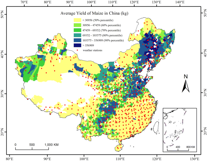
Location of 740 weather stations and distribution of the annual average total yield of maize at the county level in mainland China. The main production counties had an annual average total yield greater than the 50th percentile of the annual average total yield of all counties (light green to dark blue areas). The data were processed in MATLAB software32 version R2016a (https://cn.mathworks.com/products/matlab/). The map was generated in ESRI ArcGIS software33 version 10.2.1 (https://www.esri.com/software/arcgis/arcgis-for-desktop).
In this study, the observed maize yield per unit area (kg/ha) was used to obtain the CV. The yield per unit area time series was decomposed into three components by using the linear moving average method: the meteorological yield, the trending yield (or technical yield in some studies), and the error53,54. Ultimately, the meteorological yield was further processed to obtain the relative meteorological yield, in which the negative values were taken as the object to obtain the probability of reduction, risk index, and ICRI.
Coefficient of variation ((mathbf{C}mathbf{V}))
The CV of yield per unit area indicates the variations in yield caused by climatic and socioeconomic conditions. The equation is as follows:
$$mathrm{C}mathrm{V}=sqrt{frac{1}{mathrm{n}-1}times sum_{mathrm{i}=1}^{mathrm{n}}({mathrm{Y}}_{mathrm{i}}-overline{mathrm{Y}})}$$
(1)
where ({mathrm{Y}}_{mathrm{i}}) is the (mathrm{i})th observed yield per unit area (kg ha−1); (overline{mathrm{Y}}) is the mean of ({mathrm{Y}}_{mathrm{i}}) during the period 1981–2010; and (mathrm{n}) is the total number of observations, which is at least 15.
Meteorological yield (({mathbf{Y}}_{mathbf{w}})) and trending yield (({mathbf{Y}}_{mathbf{t}}))
The observed maize yield per unit area is impacted by natural conditions (temperature and precipitation) and socioeconomic components (technological progress and infrastructure improvements). The yield can be divided into three parts: trending yield (({mathrm{Y}}_{mathrm{t}})), meteorological yield (({mathrm{Y}}_{mathrm{w}})) and random output/error ((upvarepsilon)). The equation is as follows:
$$mathrm{Y}={mathrm{Y}}_{mathrm{t}}+{mathrm{Y}}_{mathrm{w}}+upvarepsilon$$
(2)
where (mathrm{Y}) is the annual observed maize yield per unit area. Since the random yield ε is quite small, it can be ignored. Furthermore, the simplified Eq. (1) is:
$$mathrm{Y}={mathrm{Y}}_{mathrm{t}}+{mathrm{Y}}_{mathrm{w}}$$
(3)
The approach used to simulate the trending yield has an assumption that no marked technological progress took place in the time step chosen55. Although there is no definite evidence to show the time interval of the application of new crop varieties or technologies, the Five-Year Plan in China aims for economic growth and technological development. The period of research data (1981–2010) contains six Five-Year Plans, of which 1981 is the start of the 6th Five-Year Plan and 2010 is the end of the 11th Five-Year Plan. In addition, the trending yield and meteorological yield calculated with the 5-year linear moving average method met three criteria that determine trend models56, and this method can smooth irregularities and high-frequency variations in the trends28. Thus, the five-year linear moving average method was employed to simulate the trending yield. The time series of (mathrm{Y}) was divided into sequence segments according to the time step (k), which is 5 in this study. The number of segments is (mathrm{n}-mathrm{k}+1). The linear regression for each segment ((mathrm{j})) is as follows:
$${mathrm{Y}}_{mathrm{j}}(mathrm{t})={mathrm{b}}_{mathrm{j}}+{mathrm{k}}_{mathrm{j}}times mathrm{t}$$
(4)
$$mathrm{t}=left{begin{array}{c}1, 2, 3, dots , k if j=1 2, 3, 4, dots , k+1 if j=2 vdots n-k+1, n-k+2, n-k+3, dots , n if j=n-k+1end{array}right.$$
(5)
where ({mathrm{Y}}_{mathrm{j}}(mathrm{t})) is the ({mathrm{tth}}) trend yield in segment (mathrm{j}), ({mathrm{k}}_{mathrm{j}}) and ({mathrm{b}}_{mathrm{j}}) are estimated from a set of (mathrm{Y}) and (mathrm{t}) in segment (mathrm{j}) with the least squares method, and (mathrm{t}) is the rank index of each observed year. There can be more than one simulated value for each (mathrm{t}) in segment 2 to (mathrm{n}-mathrm{k}+1). Finally, the trending yield of each (mathrm{t}) is a moving average:
$${mathrm{Y}}_{mathrm{t}}left(mathrm{t}right)=averageleft(sum_{mathrm{j}=1}^{mathrm{n}-mathrm{k}+1}{mathrm{Y}}_{mathrm{j}}left(mathrm{t}right)right) t=1, 2, 3, dots , n$$
(6)
where ({mathrm{Y}}_{mathrm{t}}(mathrm{t})) is the ({t}{text{th}}) trending yield.
$${mathrm{Y}}_{mathrm{w}}(t)= mathrm{Y}(mathrm{t})-{mathrm{Y}}_{mathrm{t}}left(mathrm{t}right)$$
(7)
where ({mathrm{Y}}_{mathrm{w}}(t)) (mathrm{Y}left(mathrm{t}right)) are the ({t}{text{th}}) meteorological yield and actual yield per unit area, respectively.
Relative meteorological yield (({mathbf{Y}}_{mathbf{r}}))
The ({mathrm{Y}}_{mathrm{r}}) values are comparable since they are not impacted by the socioeconomic component15. The corresponding equation is as follows:
$${mathrm{Y}}_{mathrm{r}}(mathrm{t})=frac{{mathrm{Y}}_{mathrm{w}}(t)}{{mathrm{Y}}_{mathrm{t}}(t)}$$
(8)
where a negative ({mathrm{Y}}_{mathrm{r}}(mathrm{t})) is defined as the ({t}{text{th}}) reduction rate3.
Average yield reduction rate ((mathbf{R}))
The average yield reduction rate ((mathrm{R})) was determined by the negative value of ({mathrm{Y}}_{mathrm{r}}(mathrm{t})). The corresponding equation is as follows:
$${text{R}} = – frac{1}{{text{n}}} times mathop sum limits_{{{text{i}} = 1}}^{{text{n}}} {text{Y}}_{{text{r}}} left( {text{t}} right);;;;;{text{when}} ;{text{Y}}_{{text{r}}} left( {text{t}} right) < , 0$$
(9)
where (mathrm{n}) is the number of negative values of ({mathrm{Y}}_{mathrm{r}}(mathrm{t})).
Risk index of yield loss (({mathbf{I}}_{mathbf{R}}))
({mathrm{I}}_{mathrm{R}}) results from the integration of different levels of reduction rates (({mathrm{R}}_{mathrm{i}})) and their probability of occurrence (({mathrm{P}}_{mathrm{i}})). The greater the value of ({mathrm{I}}_{mathrm{R}}) is, the greater the risk of yield losses.
Because the climate factors that affect crop yield exhibit a normal distribution, it is argued that the ({mathrm{Y}}_{mathrm{r}}) series should also exhibit a normal distribution. The normal distribution test was performed on ({mathrm{Y}}_{mathrm{r}}) to verify this assumption. Due to the small sample size, the Lilliefors goodness-of-fit test was chosen. For a few samples that did not fit the normal distribution, the normal conversion was conducted by the logarithmic method.
There is no fixed standard for the division of the range of ({mathrm{R}}_{mathrm{i}}). The China national standard (GB/T24438.1-2009) roughly divides ({mathrm{R}}_{mathrm{i}}) into three ranges, 0.1–0.3, 0.3–0.8, and 0.8–1, to indicate three levels of damaged crop area. The threshold values of ({mathrm{R}}_{mathrm{i}}) for identifying different levels of drought (mild, moderate, severe, and extreme drought) are 0.1, 0.2, and 0.357. A value of 0.05 was used to determine whether the crop was impacted by a disaster58. Based on the above threshold, ({mathrm{R}}_{mathrm{i}}) was divided into four ranges: (left(0,left. 0.05right]right.), (left(0.05,left. 0.15right]right.), (left(0.15,left.0.35right]right.) and (left(0.35,left.1right]right.). The equation for ({mathrm{I}}_{mathrm{R}}) is as follows:
$${mathrm{I}}_{mathrm{R}}=sum_{mathrm{i}=1}^{mathrm{n}}left({mathrm{R}}_{mathrm{i}}times {mathrm{P}}_{mathrm{i}}right)$$
(10)
Comprehensive risk index of yield loss ((mathbf{C}mathbf{R}mathbf{I}))
The (mathrm{C}mathrm{R}mathrm{I}) combines (mathrm{C}mathrm{V}), (mathrm{R}), and ({mathrm{I}}_{R}). A larger (mathrm{C}mathrm{R}mathrm{I}) means a greater risk of losses. Due to the inconsistent units of the four variables, standardization is first performed using the extreme difference method. The standardized (mathrm{C}mathrm{V}), (mathrm{R}), and ({mathrm{I}}_{R}) were calculated using the following equation:
$${mathrm{x}}_{mathrm{s}}=frac{mathrm{x}-mathrm{m}mathrm{i}mathrm{n}(mathrm{x})}{mathrm{m}mathrm{a}mathrm{x}(mathrm{x})-mathrm{m}mathrm{i}mathrm{n}(mathrm{x})}$$
(11)
where (mathrm{x}) is (mathrm{C}mathrm{V})/(mathrm{R})/({mathrm{I}}_{R}), and ({mathrm{x}}_{mathrm{s}}) is the standardized (mathrm{x}).
(mathrm{C}mathrm{R}mathrm{I}) is the comprehensive risk index without considering the area effect.
$$mathrm{C}mathrm{R}mathrm{I}=frac{1}{3}times left({mathrm{R}}_{mathrm{s}}+{mathrm{C}mathrm{V}}_{mathrm{s}}+{mathrm{I}}_{mathrm{R}mathrm{s}}right)$$
(12)
where ({mathrm{C}mathrm{V}}_{mathrm{s}}), ({mathrm{R}}_{mathrm{s}}) and ({mathrm{I}}_{mathrm{R}mathrm{s}}) are the standardized versions of (mathrm{C}mathrm{V}), (mathrm{R}), and ({mathrm{I}}_{R}). The weights of these three indicators are the same28,58,59.
Improved comprehensive risk index ((mathbf{I}mathbf{C}mathbf{R}mathbf{I})) of yield loss
(mathrm{R}), (mathrm{C}mathrm{V}) and ({mathrm{I}}_{mathrm{R}}) exhibit close positive correlations with the yield loss risk, while planting area size ((mathrm{S})) exhibits a negative correlation with this risk because the increase/decrease in the yield of a field will offset the decrease/increase in another field in the same region. The (mathrm{I}mathrm{C}mathrm{R}mathrm{I}) is the comprehensive risk index after removing the planting area effect. The main maize growing counties were divided into lowest-, low-, moderate-, high- and highest-risk areas.
The (mathrm{I}mathrm{C}mathrm{R}mathrm{I}) equation is as follows:
$$mathrm{I}mathrm{C}mathrm{R}mathrm{I}=frac{1}{3}times left({mathrm{R}}_{mathrm{s}}+{mathrm{C}mathrm{V}}_{mathrm{s}}+{mathrm{I}}_{mathrm{s}}right)times frac{1}{{S}_{s}}$$
(13)
where ({mathrm{S}}_{mathrm{S}}) is the standardized planting area size calculated using Eq. (11).
Source: Ecology - nature.com
