Particles are simulated with the Ariane software (available from http://stockage.univ-brest.fr/~grima/Ariane/doc.html,20,21) modified to include independent, age-related, vertical motion of particles22. The modified Ariane is driven by the velocity, potential temperature, T, and salinity, S, fields output from the VIKING20 configuration23 of the NEMO ocean model24.
VIKING20 hydrodynamic model: description and verification
Used here as input for the Lagrangian dispersal study was VIKING20, an eddy-rich ((0.05^{circ }) or 2 km to 4.5 km in the region of interest) ocean/sea-ice model performed under past atmospheric forcing using the CORE2 data set25 of the years 1958-2009. VIKING20 is configured on the ORCA family of tripolar grids avoiding a singularity at the North Pole26, with the (0.05^{circ }) resolution grid covering the North Atlantic two-way nested27 within a (0.25^{circ }) resolution global ocean. Model vertical discretisation is on 46 z-levels (fixed in depth) with partial cells at the bed for improved representation of bathymetry. Level thicknesses range from 6 m at the surface to 250 m at 5000 m depth (about 30 m at 250 m and 200 m at 2000 m depth). VIKING20 has been demonstrated to realistically simulate the the subpolar North Atlantic23 including details of the challenging regional and western boundary current systems28,29,30.
Like many modern ocean models, VIKING20 is optimized for the upper water column. Near-bed flows, crucial to modelling the settling phase of larval life, are typically affected by larger vertical resolution at depth, not resolving the bottom boundary layer. Also not included is the simulation of tides which would lead to locally enhanced mixing and small-scale turbulence31, 32. Nevertheless, studies simulating the dispersal of deep-sea mussels16 or methanotrophic bacteria33 have demonstrated the success of VIKING20 when compared to genetic and in situ data. Despite a general impact of temporal resolution34, variable bottom flows are well represented by five-day average fields of the three-dimensional velocities. The mean horizontal velocities are direct output from the model and corresponding vertical velocities are calculated using the model 3D continuity equation.
A direct comparison of individual modelled Lagrangian particle tracks with real-world drifter tracks is impossible – uncertainties in the initialization of the model and missing model dynamics mean that the simulated and real flow fields are never the same and Lagrangian particles in each will quickly diverge. However, when large numbers of virtual particles are released, as we do here, ensembles of particle tracks have proved adept at reproducing distributions of drifting buoys, marine litter, and nutrient concentrations35,36,37,38,39. The current generation of global- and basin-scale models at least partially resolve mesoscale eddies, and shows some success in reproducing large-scale and regional circulation patterns, and are therefore able to reproduce coherent structures, patch stretching and straining, attractors and barriers40 which impact particle dispersal.
Particle track calculations
The Ariane particle tracking code finds the analytical solution for particle pathways through model gridcells; we store the updated particle positions at 5-day intervals. Modifications have been added to Ariane to include independent, age-related, vertical motion of each tracked particle, simulating the ability of organisms to actively swim vertically or control their buoyancy. This is done by adding the ‘swimming’ velocity to the vertical velocity calculated from the model for each particle at each timestep. Near the bed, downward swimming is phased out smoothly in the next-to-bottom gridbox and set to zero in the bottom gridbox, upward swimming is phased out smoothly at the target depth and zero above this depth. Near-bed particles are still advected by the model flows, particles advected back into the model interior will resume downward swimming.
Virtual particles were spawned from the 12 ATLAS project case study sites (Fig. 1). For the ATLAS project, these case study sites were selected on the basis of: proximity to blue growth activities, the presence of ATLAS focal ecosystems (cold water corals, sponges and hydrothermal vents), and data availability (see Table 1 for details). These sites were considered suitable for the current modelling study since the site distribution incorporates the diversity of sensitive Atlantic deep-water ecosystems and follows the major Atlantic current patterns. This enables us to test our hypothesis, and study the effects of larval behaviour, in a range of dynamical regimes representative of the 200 m to 2000 m depth range, including offshore banks and seamounts, east and west Atlantic shelf slope, the mid-Atlantic ridge and shallower sites on the shelf.
At each release time, two particles were released at every VIKING20 grid node that lies within the Case Study polygon and the isobath range (Table 1), one particle from near the bottom and one at the top of each bottom grid box (between a few metres and 200 m above the bed, the different release depths had no impact on the dispersal statistics). Particles were released at 200 discrete times: one burst of particles in the middle of each season (mid-January, mid-April, mid-July, and mid-October) over 50 years of the model run from 1959 to 2008 to capture seasonal and interannual variability (not reported here). Higher frequency releases were not considered to be required as spawning times of deep-sea species are generally poorly known. The total number of particles simulated for each case study, for each behaviour, is the number in the final column of Table 1 times 400 (400 = 50 years times 4 seasons per year times 2 launch depths). Polygons for LoVe Observatory (case study 1) and East Mingulay (case study 4) only encompassed a small number of model grid points, 187 and 9, respectively, so additional particles were added to the simulations by creating new particles offset by ±0.3 index units (for both) and ±0.1 index units (only for CS04) to the particles launched exactly at the grid nodes. Rockall Bank (case study 3) and Reykjanes Ridge (case study 9) polygons contained too many points so the numbers of particles were cut down by sub-sampling every 4th node and every 10th node respectively.
From the deep-sea literature18,19, 41,42,43,44 we have identified 5 key larval vertical movement behaviours, and selected ranges of each within the bounds of observed behaviours:
- 1.
Age of maturity at which full swimming ability, or maximum positive buoyancy is reached. Range [0,10 days].
- 2.
Age of competency at which larvae start heading downwards to find somewhere to settle. Range [4 days, 42 days].
- 3.
The peak upward swim (or buoyancy driven) speed achieved after the age of maturity. Speed increases linearly from age zero until the age of maturity. Range [0.2 mm s−1, 1.0 mm s−1].
- 4.
Maximum downward speed. This is the speed of descent after the age of competency. Range [−0.2 mm s−1, −1.0 mm s−1].
- 5.
The target depth below the surface at which larvae stop heading upwards. Range [6 m, 120 m], this range was chosen to investigate the possible effects of near-surface wind-driven Ekman layer flows on particle dispersal.
In a systematic experiment, with each trait varying independently, this gives a total of (2^5 left( = 32right) ) tracking experiments each with 9.2 million active particles. The behaviours are shown schematically in Fig. 2, a full list is in Table 2. A further control data set is 9.2 million passive (purely advective) particle tracks.
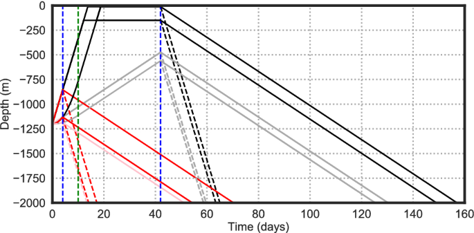
Depth versus time schematic of the 32 larval behaviours modelled (black and red lines). Vertical dashed blue lines are the age of competency. Vertical dashed green line is the later age of maturity (the earlier one is zero). Steep/shallow upward/downward gradients show the fast/slow upward/downward swimming speeds. Near-surface horizontal sections on the black lines show the target depths (many particles may never reach these levels). Many of the 32 line sections overlay each other. Once particles reach the bed they continue close to the bed. Every particle survives for 6 months (185 days).
In each run, particles were spawned quarterly over 50 years and each tracked in the model for 6 months (185 days). This duration was chosen based on a summary of published estimates18 together with recent estimates of lifespans of over 1 year for some deep-sea species19,44. We have not modelled possible larval behaviours dependent on ocean temperature and salinity. We allow particles to cross watermass boundaries freely based on laboratory44,45 and field observations46 of this behaviour.
Particle track visualization and postprocessing
Particle tracks are stored in netCDF format and the post-processing and visualization of the larval simulations has been performed in Python using NumPy, Matplotlib, and cf-python packages as well as with the tcdf particle track visualization toolkit22,47. All tracks are accumulated and at intervals of 5 days of particle ‘age’ (time since particle release), 2D (x–y) histograms of modelled particle positions are constructed using bins of ({0.25}{^{circ }}times {0.25}{^{circ }}) horizontal resolution. Two types of histograms are constructed; the first type includes all particle positions in each bin (depth-integrated) and the second type uses only the particle positions within the two bottom grid cells (depth-selective) to highlight where larvae may settle48. Area of spread is quantified as the smallest area within the contours enclosing 100%, 95%, 90%, 80% and 50% of the particle positions16. Note that the spreading areas reported in the main article and in the area metrics presented below are always based on the 95% confidence contour, the other contours are present in Supplementary Figs. S13–S24.
Particle track ensemble metrics for quantification
In order to quantify the total spreading and relative change in regime experienced by particles, we formally define two metrics that describe the time evolution of an ensemble of particle tracks (Fig. 3). The first, the area growth, G,
$$begin{aligned} G = A(text {185 days}) – A(text {0 days}), end{aligned}$$
(1)
is the difference in areas, A(t), contained within the 95% confidence contour of the depth-integrated particle position probability map after 185 days and at the time of launch. The second metric, the relative area growth curvature, is the normalized area between the curve A(t) and a straight-line diffusive approximation from (A(text {0 days})) to (A(text {185 days})), a(t),
$$begin{aligned} C = frac{int _{t=0}^{t=185} A(t) – a(t) dt}{int _{t=0}^{t=185} a(t) dt} = frac{int _{t=0}^{t=185} epsilon (t) dt}{frac{1}{2} G Delta t}, end{aligned}$$
(2)
where (epsilon (t)) is the instantaneous difference between the area growth curve and the simple diffusion reference line and (Delta t) is 185 days. Positive (or negative) values of C mean that the spreading area initially grows faster (slower) than the simple diffusive reference and then slows down (speeds up). Values close to 0 suggest that the area growth is very similar to the simple diffusive reference line with minimal change in flow regime. Since a straight line is the reference within C and there is no contraction of area with time, C is always between -1 and 1.
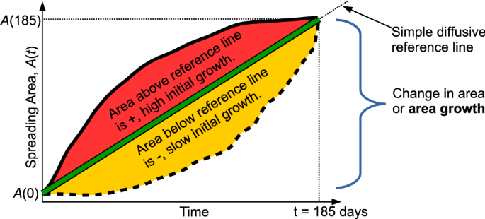
Schematic of the definition of the area growth, G, and relative area curvature, C, metrics used in quantifying particle track ensemble patterns.
Finally, for each launch site, we calculate the along-bathymetry retention after 185 days, R, for each behaviour, by dividing the number particles near the bed and between the 200 m and 2200 m isobaths (from the depth-selective histograms), by the total number of particles. This metric does not account for individual species requirements for narrower depth or temperature ranges, the heterogeneous distribution of suitable or unsuitable sea floor substrates, other environmental cues, mortality, or predation, so it is an overestimate of settling and larval survival. However, because bathymetry is the dominant filter, and ocean currents are strongly steered by bathymetry, R provides a rough quantification for the degree to which larvae follow the main currents of the Subpolar North Atlantic Ocean.
Source: Ecology - nature.com

