A model study of terraced riverbeds as novel ecosystems

Our starting point is a model for a single terrace (ecosystem) that describes a water-limited plant community^24,26. It consists of two water variables, below-ground or soil water, (W), and above-ground or surface water, (H), and biomass variables ({B}_{1},{B}_{2},ldots ,{B}_{m}), representing the above-ground biomass of (m) functional groups. We focus on functional groups of species that make different compromises in their relative investments in above-ground biomass (shoot), to capture canopy resources, and below-ground biomass (root), to capture soil resources. Specifically, we focus on two functional traits, the maximal shoot biomass (k), and the root-to-shoot ratio (E), and introduce a dimensionless tradeoff parameter (chi in [0,1]), defined implicitly through the relations:

where ({K}_{min}), ({K}_{max}) and ({E}_{min}), ({E}_{max}) determine the ranges of the two traits in the pool of functional groups, and ({epsilon }) is a positive constant (Nathan et al., 2016). Thus, (chi =0) represents a functional group that invests mostly in shoots to capture light, ((K,E)=({K}_{max},,{E}_{min})), while (chi =1) represents a functional group that invests mostly in roots to capture soil water, ((K,E)=({K}_{min},,{E}_{max})). The distributions of all other functional groups ({chi }_{i}), in between these two extremal groups, strongly depend on the value of ({epsilon }) as the tradeoff curves in Fig. 2 show.

Figure 2

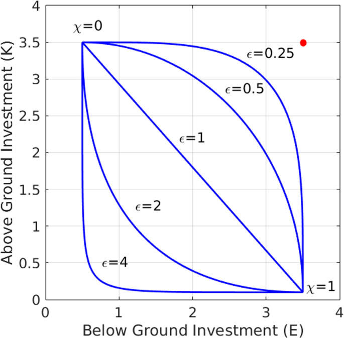
Different tradeoff curves obtained from equations (1): linear tradeoff (({epsilon }=1)), convex tradeoff (({epsilon } < 1)), and concave tradeoff (({epsilon } > 1)). The red circle denotes an “ideal functional group” (({E}_{max},,{K}_{max})) not restricted by a tradeoff. Convex tradeoffs represent pools with competitive advantage given to functional groups with intermediate χ values (closer to the red circle), while concave tradeoffs represent advantage to groups with extreme χ values, either small or large.

Full size image

The significance of ({epsilon }) can be understood by considering an ideal functional group of species (({K}_{max},,{E}_{max})), a “Darwinian demon”²⁷, that benefits from high values of both (K) and (E) (red point in Fig. 2). Functional groups that are closer to this ideal group are expected to have competitive advantage over other groups. The closest functional group can be calculated by minimizing the distance function

with respect to (chi ), where (K(chi )) and (E(chi )) are given by ((1a)) and ((1b)). For ({epsilon }=1) (linear tradeoff), such a calculation gives the intermediate value

for the closest, and thus most competitive, functional group. As ({epsilon }) is decreased below unity (convex tradeoff) a distinguished set of functional groups around ({chi }_{mid}) becomes significantly closer to the ideal group (({K}_{max},,{E}_{max})) than all other groups. By contrast, as ({epsilon }) is increased beyond unity (concave tradeoff) the distance to the ideal functional group becomes more uniform across the pool, implying a wider range of functional groups with nearly equal competitive capabilities. Note that for sufficiently high ({epsilon }) values the shortest distance to the ideal group occurs at the two extreme groups, (chi =0) and (chi =1).

The biomass variable associated with the ith functional group is ({B}_{i}=B({chi }_{i})), that is the biomass obtained by solving the model equations with the particular parameter values ({K}_{i}=K({chi }_{i})) and ({E}_{i}=E({chi }_{i})), keeping all other parameters fixed. For simplicity, we assume that in each terrace all water and biomass variables are spatially uniform. This assumption holds for homogeneous systems with weak pattern-forming feedbacks^19,28.

The terraced riverbed (meta-ecosystem) to be studied here is obtained by coupling the single-terrace models for adjacent terraces through the above-ground water variable to account for runoff contributions from upslope terraces and loses to downslope terraces. Note that we did not include sediment transport from upslope terraces as this is a secondary effect. The meta-ecosystem model for a riverbed with (n) terraces reads

where the index (i,,)runs over the (m) functional groups, the index (,j,,)runs over the (n) terraces, ({B}_{ij}) is the above-ground biomass of the i^th functional group in the j^th terrace, and ({W}_{j}) and ({H}_{j}) represent, respectively, the contents of soil water and of surface water in the j^th terrace. The factor ({Lambda }_{ij}) in equation ((1a)) is given by:

and represents growth attenuation of species that suffer from competition for light (Nathan et al., 2016). This competition is strongly affected by the maximal-shoot biomass parameters, ({K}_{i}), which affect the late-stage growth of the plant species. These parameters represent species-specific growth limitation, assumed here as resulting from self-shading, and thus related to specific leaf area. Competition for water is captured by the water-dependent biomass growth factors ({(1+{E}_{i}{B}_{ij})}^{2}{W}_{j}/(1+a{W}_{j})) in Eq. (1a) and by the water-uptake rates (sum _{i}{varGamma }_{i}{B}_{ij}{(1+{E}_{i}{B}_{ij})}^{2}) in Eq. (1b). That competition is strongly affected by the root-to-shoot ratios, ({E}_{i}), of the different functional groups. The source of soil water ({W}_{j}) in any terrace comes from the infiltration of surface water ({H}_{j}) at a rate (I). The source of surface water comes from precipitation at a time-dependent rate (P) and runoff contributions from adjacent upper terraces and from surrounding hillsides. The latter contribution often comes predominantly from the hillslopes that surround the uppermost terrace (j=n) and is modeled in Eq. (2d) by the term (alpha P), where (alpha ) is a function of the precipitation rate given by

This form captures the diminishingly small runoff contribution at low (P) when the soil is dry, (alpha Papprox {alpha }_{1}{P}^{3}ll P), the surge in that contribution as (P) increases, and its attenuation at high (P), as the soil becomes saturated and the runoff-contribution approaches a linear dependence, (alpha Papprox (frac{{alpha }_{1}}{{alpha }_{2}})P), with a proportionality factor (frac{{alpha }_{1}}{{alpha }_{2}}) that reflects the watershed. The runoff coupling between adjacent terraces is introduced through the terms (D({H}_{j+1}-{H}_{j})) in Eq. (2c), where the parameter (D) provides a measure for the coupling strength. An illustration of the factors that affect surface-water dynamics in a terraced riverbed is shown in Fig. 3.

Figure 3

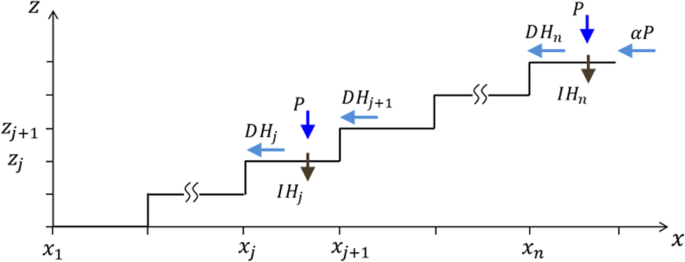
An illustration of surface-water dynamics in terraced riverbed. Gain of surface water in the jth terrace is due to precipitation, (P), and runoff contribution, (D{H}_{j+1}), from the adjacent upper terrace. Loss of surface water in the jth terrace is caused by infiltration into the soil, (I{H}_{j}), and by runoff, (D{H}_{j}), to the adjacent lower terrace. The uppermost terrace receives a runoff contribution, (alpha P), from the surrounding hillslopes.

Full size image

The reader is referred to Table 1 for a list of all model parameters, their meanings, units and numerical values. A few more comments are in order. We assumed that the biomass loss parameter ({M}_{i}), which represents mortality and additional factors such as grazing, is uniform across the community ({M}_{i}=M). This is unlike an earlier study²⁰ where a distinction between short and long grazing histories was made. We have not modeled transport of soil water between the terraces as it is much slower that the transport of surface water⁸. We have not included an evaporation term in the surface-water Eq. (2c,d) because of the fast conversion of surface water to soil water through infiltration. For simplicity, the runoff rate (D) is considered to be a constant. In practice, runoff is slowed down by vegetation and (D) is biomass dependent. We note that (D) is related to the uniform extension (l={x}_{j+1}-{x}_{j}) of the terraces and to their uniform height (d={z}_{j+1}-{z}_{j}) (see Fig. 3) through (propto frac{d}{{l}^{2}}).

Source: Ecology - nature.com