Calculations for hypothetical scenarios
In a forest comprising three taxonomic groups, the overall fractional mortality, M, of all trees in height class i is given by
$$M_i = (d_{i,1} + d_{i,2} + d_{i,3}){mathrm{/}}(n_{i,1} + n_{i,2} + n_{i,3}),$$
(1)
where ni,1, ni,2, and ni,3 are the numbers of living trees in height class i and taxonomic groups 1, 2, and 3 at the start of the measurement period, and di,1, di,2, and di,3 are the numbers of those trees that died by the end of the measurement period. Thus,
$$M_i = d_{i,1}{mathrm{/}}(n_{i,1} + n_{i,2} + n_{i,3}) + d_{i,2}{mathrm{/}}(n_{i,1} + n_{i,2} + n_{i,3}) + d_{i,3}{mathrm{/}}(n_{i,1} + n_{i,2} + n_{i,3}),$$
(2)
$$,,,,, = (d_{i,1}{mathrm{/}}n_{i,1})left( {n_{i,1}{mathrm{/}}(n_{i,1} + n_{i,2} + n_{i,3})} right) + ( {d_{i,2}{mathrm{/}}n_{i,2}} ) left(n_{i,2}{mathrm{/}}(n_{i,1} + n_{i,2} + n_{i,3})right) ,,, + (d_{i,3}{mathrm{/}}n_{i,3})left( {n_{i,3}{mathrm{/}}(n_{i,1} + n_{i,2} + n_{i,3})} right),$$
(3)
$$ = m_{i,1}p_{i,1} + m_{i,2}p_{i,2} + m_{i,3}p_{i,3},$$
(4)
where mi,1, mi,2, and mi,3 are the fractional mortalities of trees in height class i and taxonomic groups 1, 2, and 3 over the observation period, and pi,1, pi,2, and pi,3 are the proportions of living trees in those taxonomic groups relative to all trees in height class i at the start of the observation period. That is, pi,1 + pi,2 + pi,3 = 1. As described in “Analysis” section (below), Eq. (4) was used to calculate hypothetical mortality of all trees within height classes for Fig. 1d, Supplementary Fig. 2, and Supplementary Tables 4 and 5.
Reflecting our paper’s main analyses, Eq. (4) assumes three taxonomic groups, but generalizes to
$$M_i = m_{i,1}p_{i,1} + ldots + m_{i,x}p_{i,x},$$
(5)
where x represents any number of taxonomic groups ≥2. Equation (5), with x = 2, was used to calculate mortality of all trees within height classes for our hypothetical examples illustrating the two introductory scenarios (Supplementary Tables 1 and 2).
Data
Details on data collection can be found in ref. 2; here we provide a brief summary. Within a 1705-ha forested landscape (1524–1829 m elevation), locations of our 89 0.1-ha plots were selected a priori using Generalized Random Tessellation Sampling (GRTS), which provides a spatially balanced sample that has a true probability design10. Within each plot, we recorded the species, trunk diameter at breast height (DBH; breast height = 1.37 m) by 5-cm classes, and condition (living or dead) of all standing conifers >0 cm DBH and all standing angiosperms ≥5 cm DBH. Each dead tree was further classified according to its foliage and fine twig retention to allow estimation of timing of death (see “Analysis” section, below). Data were collected in Microsoft Access (version 2016) using Microsoft Access forms.
Height classes of individual trees (5–15 m, 15–30 m, and >30 m, following Stovall et al.1) were estimated from DBH using published species-specific allometric equations (Supplementary Table 3). Sources of equations were selected for geographic proximity to our study site and for large numbers of calibration trees spanning a broad range of heights. Because DBH of our trees was recorded in 5 cm classes, DBH thresholds between height classes were assigned to the nearest 5 cm DBH (Supplementary Table 3). Although different sets of allometric equations undoubtedly would yield somewhat different species-specific thresholds among height classes, our broad conclusions would almost certainly remain unchanged; for example, the same size-related patterns of tree mortality that we found relative to tree height (Fig. 1b; Supplementary Fig. 1) are also evident relative to trunk diameter2.
Analysis
Mortality was calculated as in ref. 2, with the exception that because our primary goal was to explore the consequences of taxonomic groups on the overall mortality of a sample, we simplified the model by excluding plot as a random effect. We first calculated the probability that a given tree died prior to 2014. The data allowing us to do this came from other plots where, extending back decades, we knew the exact years of death for 2297 standing dead trees. In the summer of 2016, we classified each of these 2297 dead trees according to the same foliage and fine twig retention classes we used in the 89 randomly located plots, allowing us to fit probability distributions (gamma distributions) for year of tree death as functions of species and foliage or twig retention class. When we lacked adequate samples for some less-common tree species, we used the probability distributions of similar taxa, as follows: Abies magnifica and Torreya californica used A. concolor calibration; Pinus jeffreyi used the combined P. ponderosa + P. lambertiana calibration; and all angiosperms used the Quercus kelloggii calibration. The probability distributions were then used to calculate the probability that each tree in our 89 randomly located plots died prior to the drought. Given that probability, which allows us to incorporate year-of-death uncertainty into our credible intervals, we then fit a logistic model to estimate the probability that a tree of a given taxonomic group and height class died in 2014–2016. All parameters were fit as part of Bayesian models using a Markov Chain Monte Carlo approach, with parameters having either diffuse normal or diffuse uniform (uninformative) priors, as detailed in ref. 2. We used three chains (unthinned) and for each chain used 20,000 iterations, with 5000 of those iterations used as burn-in. For all Bayesian analyses (including the determination of gamma distributions above), we examined traceplots of the chains to detect obvious lack of convergence, excessive autocorrelation, poor mixing, or inadequate burn-in. Convergence was also evaluated using the Gelman–Rubin diagnostic; in all cases, the Gelman-Rubin diagnostic was very near 1, indicating good convergence. Analyses were performed using R 3.6.2 with the coda 0.19.3, rjags 4.10, and R2jags 0.5.7 packages in combination with JAGS 4.3.0 software (Supplementary Code).
Within each height class i and taxonomic group t, we estimated numbers of trees that were alive in 2013 as
$$n_{2013,i,t} = n_{2016,i,t}{mathrm{/}}(1 – m_{i,t}),$$
(6)
where n2016,i,t is the actual number of living trees we recorded in height class i and taxonomic group t during our 2016 field surveys, and mi,t is the corresponding 2014–2016 fractional mortality, estimated as described in the preceding paragraph. Estimated numbers of trees that died 2014–2016 were then calculated as
$$d_{i,t} = n_{2013,i,t} – n_{2016,i,t}.$$
(7)
Numbers derived from Eqs. (6) and (7) are presented in Supplementary Table 6 and Supplementary Fig. 3, and were used to calculate the various proportions, pi,t, shown in Supplementary Tables 4 and 5, and in associated figures.
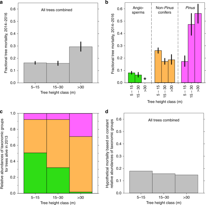
To derive Fig. 1d, we used Eq. (4) to calculate hypothetical mortality for all trees considered together within each height class, using actual height- and taxa-specific mortality values (Fig. 1b) but assuming constant abundances of taxonomic groups (those of the population as a whole) across the three height classes for trees alive in 2013 (Supplementary Table 4). (Because they represent numbers of trees alive in 2013, these proportions differ slightly from what would be calculated from the numbers in Supplementary Table 3, which represent all living and dead trees in our sample regardless of year of death.) Similarly, we wished to explore the second introductory scenario: even though Pinus comprised only ~10% of trees, its increasing mortality with height must also have contributed to the overall increase in tree mortality with height shown in Fig. 1a. We thus used Eq. (4) to calculate hypothetical mortality for all trees considered together within each height class, but this time using actual relative abundances of taxonomic groups within height classes, and actual height- and taxa-specific mortality values for angiosperms and non-Pinus conifers, but assuming constant Pinus mortality (that of the Pinus population as a whole) across the three Pinus height classes (Supplementary Table 5).
Reporting summary
Further information on research design is available in the Nature Research Reporting Summary linked to this article.
Source: Ecology - nature.com
