Study area
The study was conducted in a tropical rainforest in Babatngon Range in the northeastern portion of Leyte Island (Fig. 7) which covers two municipalities- San Miguel and Babatngon. The core of the mountain range is represented by ultramafic outcrops known as the Tacloban Ophiolite Complex (TOC). It is a NW–SE trending massif in the northeastern portion of the island, overlain by sedimentary sequences dated to Late Miocene-Pliocene and Pleistocene volcaniclastic deposits on its eastern and western flanks, respectively43. The maximum elevation of the study area reaches up to 600 m a.s.l with an average elevation range from 19.67 to 197.88 m a.s.l and with a median and interquartile range (iqr) of 68.50 (102.00 m a.s.l.). Under the Modified Corona’s Climate Classification System, the study area has a Type IV climate characterized by having no dry season and more or less evenly distributed rainfall throughout the year44,45. The warmest month is April with an average temperature of 28.1 °C and the pronounce wetness occurs in the months of November, December, and January with rainfall of 279.0 mm, 305.3 mm, and 281.17 mm, respectively46. Like in many tropical forest ecosystems, the predominant causes of forest degradation in the hilly portions of the study area were the slash-and-burn agriculture (“Kaingin”) which involves clearing and burning of forests for agricultural purposes, and illegal logging. Whereas the lowlands are already converted to rice paddies which are mostly rain fed. These resulted in the degradation and alterations of forest ecosystems in the study area.
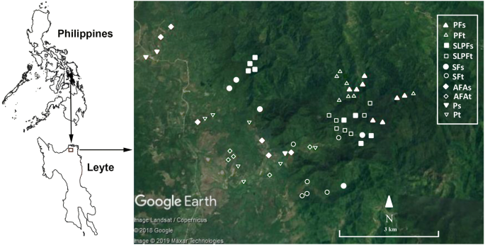
Map of the area and study plots in a lowland tropical rainforest in northeastern Leyte, Philippines. PF primary forest, SLPF selectively logged primary forest, SF secondary forest, AFA abandoned farm area, P pasture; s stream, t terrestrial habitats.
Sampling sites
Prior to the sampling, ground surveys were conducted by visiting the study area to identify the habitats for amphibian sampling, these included primary forest (less altered), selectively logged primary forest, secondary forest, abandoned farm areas and pastures (highly altered), representing a gradient of habitat alteration. In addition, informal interviews with the local residents and owners were conducted to know the land use histories of the study sites selected. All the forest types included in this study were all contiguous.
Primary forest
The primary forests are considered to be less disturbed having no significant human disturbance primarily logging. Primary forests tend to be located in protected watershed areas and in areas with very steep terrain. These primary forests are characterized by unlogged and intact dipterocarp forests with canopy reaching 30–50 m high. The intent to sample pristine and undisturbed forest was complicated by the fact that much of the primary forests in the study area have already been subjected to minor disturbance such as rattan harvesting and wildlife hunting and collection (e.g. wild pig, birds and orchids).
Selectively logged primary forest
The selectively logged primary forests were characterized by traces of old and newly cut trees, as well discarded woods were commonly observed along the streams. These logged forests had very few or no remaining dipterocarps although some other large trees could still be observed. In addition, these forest areas were also frequently subjected to rattan harvesting and wildlife hunting.
Secondary forest
The secondary forests varied from 5 to 15 years old. All secondary forest stands have similar past land use, having been cleared for agricultural purposes, and have regenerated since abandonment. The vegetation composition of the secondary forests was predominantly characterized by early successional and fast growing trees species (e.g. Commersonia bartramia, Ficus spp. and Piper aduncum) and large long-lived pioneer species (e.g. Artocarpus sp. and Cananga odorata). However, some remnants of agricultural crops (e.g. banana and coconut) were still observed in these areas.
Abandoned farm area
The abandoned farm areas were characterized mainly by grasses with bushes like melastoma (Melastoma sp.) and guava plant (Psidium guajava). Although few tree species might be present including the exotic Gmelina tree (Gmelina arborea). Few of the abandoned farm areas were very seldom subjected to grazing.
Pasture
The pasture areas sampled in this study are permanently grazed, and are usually adjacent to abandoned farm areas or forest remnants. The pasture areas are typically either abandoned paddy fields or subsistence crops. These areas are marked by the sparse presence of trees or bushes, with a thin layer of grasses.
Amphibian sampling
To sample amphibian species, a total of 62 unique 2 m × 50 m strip plots6,9,35 were laid with 15 strip plots in the primary forest (8 stream and 7 terrestrial strip plots), 15 in selectively logged primary forest (8 stream and 7 terrestrial strip plots), 11 in secondary forest (5 stream and 6 terrestrial strip plots), 11 in abandoned farm areas (6 stream and 5 terrestrial strip plots) and 10 in pastures areas (3 stream and 7 terrestrial strip plots). To sample stream breeding amphibians, 1 m wide riparian vegetation in both banks of the stream including the water body were searched. As well, a 2 m wide strip plots in the terrestrial (interior) were laid 50 m away from the nearest stream whenever possible9. Similarly, stream strip plot of the same dimension were laid in non-forest habitats (abandoned farm areas and pasture) and we made sure that the section of the stream had the same habitat type for both banks. The terrestrial strip plots were usually close and parallel to trail, in case of abandoned farm areas. The strip plots were generally straight linear however, deviated wherever there were obstacles, or paths were constrained by topography, and stream pattern. The strip plots were placed away from habitat edges as much as possible, though sometimes they could not be avoided in small forest areas (particularly in the young secondary forests). The distance between the strip plots was kept to a minimum of 300 m in forest sites and 200 m in non-forest sites. To maximize sampling independence, only one strip plot in each patch of non-forest habitat (abandoned farm areas and pasture) was established, and each separated by stream or forested area. Also, to minimize the seasonal confounding effects, different combinations of strip plots from the different habitat types were sampled throughout the sampling period36 whenever possible. All the strip plots were positioned using a hand-held GPS (Garmin etrex).
The amphibian sampling took place from November 2017 to December 2018. This study used only visual encounter survey9,31,41 whereby each strip plot was thoroughly searched for amphibians twice in the same day, first in the morning at 0800 to 1100 h, and second in the night at 1900 and 2200 h (in order to sample both diurnal and nocturnal species). Since only visual encounter survey was employed, only leaf-litter and semi-aquatic amphibians were effectively sampled, though all guilds of amphibians encountered were recorded. All the strip plots received a second session of day and night sampling in the same day, in at least one week, thus every strip plot received a total of four sampling sessions9. In this study, a total of 248 sampling sessions were conducted. Two people (with head torch for night sampling) slowly progressed at ground level and thoroughly searched and recorded every amphibian species that were encountered and captured. This included searching numerous kinds of substrates or surfaces such as leaf litter, rocks, soil, fallen or rotten logs, shrubs, tree trunks, branches and leaves27. Amphibian surveying was limited vertically to 3 m above ground level, which generally represents a restriction in the surveyors’ ability to detect individuals. The speed of the sampling per plot was approximately 3 m/min except during handling and recording. A total of two to three strip plots were sampled for each day and night survey depending on the topography and distance between strip plots except for one occasion where only one strip plot was sampled. To minimize the disturbance in the study system, logs were not displaced and plants were not cut or uprooted except when there were vines obstructing the transect. All individuals captured were marked via toe clipping47 and measured for snout-vent length (SVL) in mm. The individuals sampled were released unharmed at the point of collection after taking measurements and photographs.
Amphibians sampled in the field were identified and photographed for vouchering. Amphibian species were identified following existing relevant literature on Philippine amphibians18,19,24 particularly for the Mindanao PAIC and as well AmphibiaWeb48 and International Union for the Conservation of Nature (IUCN) red list criteria28 were consulted for further verification.
Environmental variables
Environmental variables such as elevation, DBH, tree height, tree density, air temperature, understory density, leaf litter thickness, and leaf litter volume were measured to determine whether they affect the pattern of amphibian assemblage particularly leaf-litter and semi-aquatic species in the different habitat alteration types and habitat types. The elevation of each strip plot was recorded from a handheld GPS reading (accuracy: ± 3 m). All the trees with a DBH of ≥ 5 cm along the strip plots with a total area of 100 m2 were sampled. The total number of trees was counted as well as DBH was measured and the tree height was visually determined through the use of a 2-m long calibrated pole49. The values for DBH and tree height were averaged for each strip plot. Air temperature at each strip plot was measured using a thermohygrometer (accuracy: ± 1 °C) after 10 s of exposure for the two day sampling period. The understorey density was measured by placing a 2-m-long pole with a diameter of 2 cm perpendicular to the ground at the center of the strip plot in the interior forest, and the number of leaves touching the pole was counted9. The thickness of leaf litter was determined by inserting a sharpened wooden dowel (3 mm diameter) into the litter. The top portion of the litter was marked along the wooden dowel and the surrounding leaf litters were removed aside until reaching the humus layer of the soil. Afterwards, the difference between the soil layer and the marked portion of the wooden dowel was measured using a graduated ruler50. Determining leaf litter volume was carried out by collecting leaf-litter from an area of 1 m2 and pressing the leaf litter samples in a bucket of known volume (5,000 cm3) and measuring the height (cm) of the column51. The measurements for air temperature, understorey density, leaf litter thickness and leaf litter volume were done at an interval of 10 m along the strip plot and the values were averaged also. The environmental parameters (understorey density, leaf litter thickness and volume) were measured for both banks for stream strip plots.
Data analysis
The abundance (total number of individuals encountered/recorded), species richness and diversity of leaf-litter and semi-aquatic amphibians were determined for each strip plot across habitat alteration types (primary forest, selectively logged primary forest, secondary forest, abandoned farm areas and pasture) and for every habitat type (stream and terrestrial). Individual rarefaction curves were generated to illustrate the pattern of species richness and adequacy of sample size among habitat alteration types for stream and terrestrial strip plots. Diversity index and rarefaction curves were calculated using the PAST 3.2252. Presence of autocorrelation in spatial data is a common issue that indicates dependence between observations53, hence, spatial autocorrelation analysis (Moran’s I) was performed in R package ape54. The Moran’s I test was performed for the data on abundance, species richness and diversity by using the mid-point geographical coordinates of each strip plot. Though Moran’s I test for all the variables were significant, the Moran’s I values were very close to 0 (Supplementary Table S3) suggesting very minimal spatial autocorrelation55.
Spearman’s correlation was performed to determine correlated and non-correlated environmental variables. To study the differences in measured environmental variables and to confirm the a priori classification of habitat disturbance, Kruskal–Wallis ANOVA was performed for both stream and terrestrial habitats separately. Generalized linear models (GLMs) were carried out to assess the effects of habitat alteration types (primary forest to pasture) and habitat types (stream and terrestrial) including their interactions to amphibian abundance, richness and diversity. The GLMs analysis used poisson distribution with logarithmic link function for count data (abundance and richness) whereas normal distribution with identity link function was used for continuous data (diversity). In addition, the ratio between the degrees of freedom (df) and deviance of all the models were below 2.5 indicating acceptable model fit. Both the Kruskal–Wallis ANOVA and GLMs analysis were performed using SPSS 20 for Windows.
The non-metric multidimensional scaling (NMDS) ordination was applied to explore the variation of amphibian assemblage across the different habitats14,30,35. For this study, NMDS was performed whereby the ordination was constructed from the Bray–Curtis dissimilarity matrix of pairwise dissimilarities between transects based on abundance data. The NMDS was performed using the function “metaMDS” from R package vegan56. In constructing the ordination diagram, twenty random starting configurations were used, with the final configuration that minimized the stress of the ordination configuration retained for plotting. The NMDS ordination projects the multivariate data into a space with a smaller number of dimensions. They are arranged in space in such a way that the most similar sites are close together, while sites that are more different are further apart36. The Analysis of Similarities (ANOSIM) permutation tests in vegan package of R56, with 5,000 random permutations of the dissimilarity matrix was performed to test the differences in species assemblage of leaf-litter and semi-aquatic amphibians across habitat alteration types for stream strip plots.
To explore the relationship between the distribution of leaf-litter and semi-aquatic amphibian species and environmental variables in a gradient of habitat alteration, linear vectors were fitted into the NMDS ordination using the function envfit in the vegan package of R56. This was done by running first an NMDS ordination of species and then followed by fitting the linear vectors (environmental variables) simultaneously. The analysis used the same species abundance data, and environmental variables fitted into the ordination included elevation, tree density, tree height, DBH, temperature, leaf litter thickness, leaf litter volume and understory density. The significance of the environmental vectors was evaluated using a permutation test with 1,000 random permutations.
Lastly, the relationship between the abundance, species richness and diversity of leaf-litter and semi-aquatic amphibians with environmental variables were examined using the Generalized Additive Model (GAM) in R package mgcv57. The GAM performed for abundance and species richness (count data) used Poisson error structure and logarithmic link functions while Gaussian error structure and identity link function for diversity (continuous data). All the environmental variables with correlations > 0.65 were excluded in the analysis, thus, only understorey density, tree density, temperature and DBH were considered.
In performing the GAM, a full model was first fitted with smooth-terms for all the selected environmental variables. With the initial fitting, some of the environmental variables were best fitted by smoothed-terms with effective degrees of freedom (edf) equal to one indicating simple linear relationships. Thus, in the succeeding fitting, these terms were expressed into linear terms. The final model was selected by dropping the least significant environmental variables one at a time until the Akaike’s Information Criterion (AIC) no longer improved. In addition, residual plot for each of the model was also checked. The shape of the response curves associated with each term was illustrated by plotting the partial effects.
The NMDS, ANOSIM, fitting of linear vectors and GAM analyses were only performed for habitat alteration types for the stream strip plots with the use of R software version 3.4.358. This was due to insufficient samples (species counts or abundance) for terrestrial habitat type. In addition, due to limitation in sampling methodology used wherein visual encounter survey was only performed, some arboreal species were probably missed. Thus, we excluded arboreal species in all the statistical analyses and focused only on leaf-litter and semi-aquatic species. Also, singletons were excluded in all the analyses.
Source: Ecology - nature.com
