Long-term observations from Antarctica demonstrate that mismatched scales of fisheries management and predator-prey interaction lead to erroneous conclusions about precaution

Strata

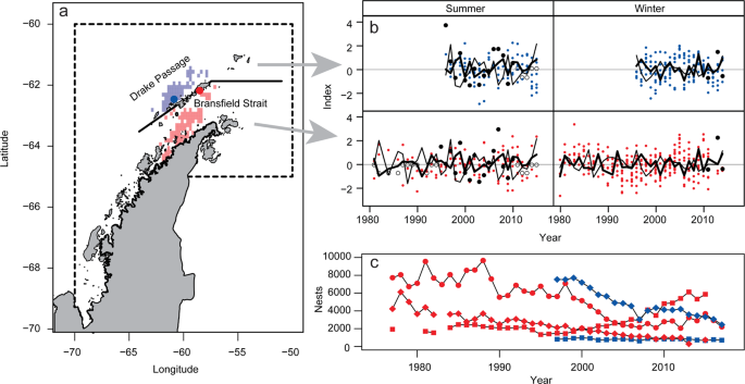
We defined two geographical strata to spatially match season-specific penguin foraging locations with estimates of LKB and LHR. These strata were based on areas where foraging penguins and krill fishing overlap²⁶ and on the availability of krill biomass estimates from research-vessel surveys^22,23. We defined the strata as the Drake Passage, combining the western and Elephant Island survey strata of the U.S. AMLR Program²², and the Bransfield Strait (Fig. 1a, adapted from²⁶).

Predictors

We quantified variation in LKB using long-term acoustic survey data^22,23 from the AP collected following standard protocols^46,47. We computed the density (g/m²) of krill for each nautical mile of survey effort, computed the average density within each stratum, and multiplied those averages by the area of each stratum. Summer surveys were conducted in January and February; winter surveys were conducted in August and September. When more than one survey was conducted in a single season (e.g., January and February of the same year), we averaged the biomass estimates from those surveys. Summer surveys cover the period 1996-2011 (Fig. 1b). Winter surveys are available for 2012, 2014, and 2015 (Fig. 1b).

We computed LHRs by matching catches with temporally and spatially coincident estimates of LKB. Catch data were provided by the Secretariat for the Commission for the Conservation of Antarctic Marine Living Resources. We summed these data by season and stratum and computed LHR as local catch/LKB.

We used two climate indices to characterize seasonal variation in environmental conditions (Fig. 1b). We averaged monthly values of the Southern Annular Mode (SAM⁴⁸) for winter (April-September) and summer (October-March) indices. We also computed seasonal averages of the Oceanic Niño Index (ONI)⁴⁹. We assigned summer averages of the SAM and ONI to the second calendar year of the split year in each austral summer (e.g., the average value for October 2004 – March 2005 was assigned to 2005).

We categorized all four predictors. When the SAM is in a positive (negative) phase, westerly winds are stronger and shifted towards the pole⁵⁰, with a resulting increase (decrease) in air temperature⁵¹ and precipitation⁵² on the western side of the AP. We thus categorized the SAM according to its sign. The ONI defines La Niña and El Niño events when sea-surface temperature anomalies near the equator are respectively ≤−0.5 °C and ≥0.5 °C. Such events interact with the SAM to affect primary production and krill near the Antarctic Peninsula¹⁵, so we binned the ONI into three categories (ONI ≤ −0.5 °C; −0.5 °C < ONI < 0.5 °C; and ONI ≥ 0.5 °C) using these two temperature thresholds. Estimates of LKB are imprecise²² and may be biased by a variety of factors, including the throughput of krill through our strata⁵³. Nevertheless, the surveys distinguish periods of relative krill scarcity and abundance. Acoustic estimates of LKB ranged in magnitude from 10⁴ to 10⁷ t. In contrast, krill catches taken within our strata were reported by fishing vessels, treated as known, and ranged in magnitude from ≤10³ to 10⁵ t. Given differences in the uncertainties and magnitudes of local biomasses and catches, we categorized estimates of LKB using a threshold of 1 × 10⁶ t (1 Mt) and of LHR using thresholds of 0.01 and 0.1. The threshold for LKB evenly splits the observed orders of magnitude in krill biomass, and that for LHR provides three categories of fishing that reflect low harvest rates, harvest rates up to that used to set catch limits for krill (0.093), and fishing above that level.

Response – penguin performance

We used monitoring parameters based on observations collected during 1982-2016 at two field camps in the South Shetland Islands to quantify variations in penguin performance. Unless otherwise noted, methods of data collection have been described previously^20,54. All methods were performed in accordance with relevant guidelines and regulations, including field methods that were reviewed and approved by the University of California San Diego Institutional Animal Care and Use Committee (ID: S05480) and authorized under U.S. Antarctic Conservation Act permits (ID: ACA 2017-012). Some parameters reflect winter conditions (mean clutch-initiation date, mean female and male masses at lay, mean egg density, and relative cohort strength; Fig. 1b). Other parameters reflect conditions during the summer breeding season (fledgling mass, foraging-trip duration, and post-hatch breeding success; Fig. 1b). In all but one case, these parameters integrate over days to months. Relative cohort strength integrates over a period ≥1 year, but we assumed that most of its variation is attributable to survival during the first few months of independence²⁰. We transformed mean clutch-initiation dates and foraging-trip durations so that larger values would indicate better performance. The former parameter was transformed to days prior to 31 December (earlier clutch initiations indicate better performance); the latter was transformed to hours <60 hours (shorter trips indicate better performance). Relative cohort strength (proportion of banded penguins resighted in their breeding colonies) and post-hatch breeding success (proportion of chicks crèched) were logit-transformed. Mean egg density was calculated from the total mass and volume of eggs from 2-egg clutches. Egg data were collected during the first week after clutch completion by weighing and measuring the maximum length and width of each egg from 50 nests per species. Egg volume was estimated from its empirical relationship⁵⁵ to egg length and width. We standardized the penguin performance indices specific to each combination of monitoring parameter (transformed or otherwise), species, and site to have zero mean and unit variance (Fig. 1b).

We matched penguin-performance indices to estimates of LKB and LHR in the Bransfield Strait or Drake Passage strata using results from multi-year tracking studies that identify when and where penguins foraged²⁶. We matched the winter and summer performance indices for Adélie and gentoo penguins breeding at Copacabana (Fig. 1a, adapted from²⁶) with LKB and LHR in the Bransfield Strait. We matched winter indices for chinstrap penguins breeding at Cape Shirreff (Fig. 1a, adapted from²⁶) with LKB and LHR in the Drake Passage, while those for gentoo penguins breeding at the same site were matched with predictors in the Bransfield Strait. After matching, we pooled performance indices within 18 bins defined by all combinations of the categorized predictors.

Model

We fitted an analysis of variance model with two components. The first component imputes missing estimates of LKB because krill surveys were not conducted every year. We modeled LKB as a function of stratum and the sign of the SAM during summer.

({K}_{ij}) is the expected value of (mathrm{ln},LKB) in stratum (i) given sign (j) of the SAM during summer, and ({phi }^{2}) is the variance of (mathrm{ln},LKB). We truncated this likelihood with a lower limit equal to the catch taken from stratum (i) (so (LK{B}_{ij}) would not be less than ({{rm{catch}}}_{i})) and an upper limit equal to 100 Mt (so (LK{B}_{ij}) would be less than twice the estimate of krill biomass used to manage the krill fishery⁴⁶). We used results from the acoustic surveys to specify prior distributions for the imputation model.

({bar{k}}_{ij}) is the mean (mathrm{ln},LKB) computed from survey observations in stratum (i) given sign (j) of the SAM, and ({s}_{ij}) is the standard deviation of these log-biomass estimates. We predicted missing estimates of LKB ((LK{B}_{ij}^{ast })) from Eq. (1) using the sign of the SAM for summers when acoustic surveys were not conducted. Missing estimates of LHR, denoted as (LH{R}^{ast }), were estimated from (,LK{B}_{ij}^{ast }).

We did not impute missing values for winter.

In the second component of our model, we treated all indices of penguin performance as exchangeable observations, and modeled performance ((P)) as a function of categorized ONI ((o)), LKB ((b)), and LHR ((h)).

(P) is the expected performance, and ({sigma }^{2}) is the residual variance in performance. (alpha ) quantifies mean performance across the set of predictor categories, and the parameters ({beta }_{1},{beta }_{2},,{beta }_{3},{beta }_{4},,{rm{and}},{beta }_{5},)quantify the degree to which each predictor causes expected performance to deviate from this mean. We specified prior distributions that limit inference to the study populations and the predictor bins considered here.

We specified a half-Cauchy prior distribution for the standard deviation of penguin performance and a uniform hyperprior for the scale parameter ((omega )) of the half-Cauchy^56,57.

We specified a design matrix with sum-to-zero contrasts that carries uncertainties in (LK{B}^{ast }) and (LH{R}^{ast }) through the model.

We used JAGS⁵⁸, via R⁵⁹, to sample from the posterior distributions of the model parameters. After 250,000 adaptive and 500,000 burn-in iterations, we sampled 5,000 points (retaining values from every 25th iteration during a further 125,000 iterations) from the posterior distributions characterized by three Monte Carlo chains initiated at different points in the parameter space. We evaluated our model with a variety of diagnostics. Diagnostics, data files, and the code needed to replicate our analysis are provided as Supplemental Information. Three R packages are needed to run our code: rjags⁶⁰, coda⁶¹, and ggmcmc⁶².

Source: Ecology - nature.com