Classifying the tree-level dataset
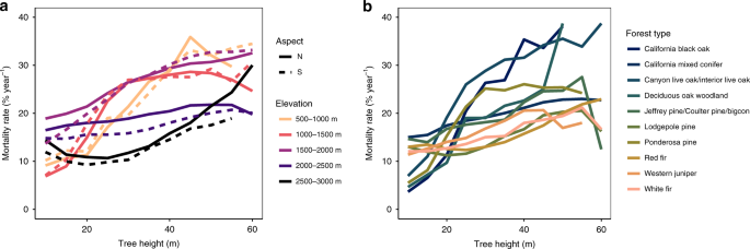
The Sierra Nevada mountains have unique species assemblages following strong topographic gradients, with the most dominant shifts controlled by topography12,13. In the low elevations the canopy is dominated by pines, shifting to fir species in high elevations. South-facing slopes tend to be dominated by drought-tolerant species, while North-facing slopes hold species more suited for cooler, wet conditions. We control for species groups by testing the height–mortality trend on our full tree-level dataset (n = 1,808,334 total; n = 656,145 trees >30 m tall), subset by [1] broad topographic drivers of species, and [2] a more complex, modeled forest type map13. Using the topographic data calculated in our original analysis1, we categorize trees into ten topographic positions: the nearest 500 m elevation bands (500–2500 m) and the North or South-facing slope (270–90° and 90-270°, respectively).
Next, we associate the USFS Forest Inventory and Analysis (FIA) forest type map13 with each tree in our dataset2. The forest type map is a predictive map of forest type, based on every FIA plot available and a suite of environmental variables. Though the local accuracy of the forest type map is not exceptional (training = 89.5%; testing = 51.0%), especially along transitions, this approach should effectively capture broad swaths of similar species for the purposes of our analysis. In total, our study area has a total of 14 forest types, but we exclude 4, due to limited total area or a lack of data in multiple height classes, limiting our inference of the full mortality–height trend. While neither of these methods distinguishes species at the scale of tree crowns, they should be telling of height–mortality trends within this ecosystem’s common species groups.
Simulating stratified plot-level data from the full dataset
We simulate 1000 different plot placement strategies using our full tree-level dataset2 and an identical plot sampling approach as Stephenson and Das. We stratified 89 circular 0.1-ha plots with a probability-based design using the categories defined in our prior analysis: [1] topographic position and [2] forest type. At each simulation step, 89 stratified plot locations are randomly selected using the grts function in the R package spsurvey. Total sample locations are determined by the proportion of area attributed to each topographic or forest type class. A simulated plot is created as a 0.1-ha subset of tree crowns identified in our original study1.
To ensure our plot-simulations were comparable to Stephenson and Das’ field data over the 5–60 m tree height range, we directly compare the average number of tree samples (dead and total) across all simulations with the field plot distributions with respect to height class (Supplementary Fig. 2). We also test the same plot simulation approach in a contiguous subset of our broad study area between 1524 and 1829 m in elevation, where mean slope was ~31° (compared to ~24° in Stephenson and Das’ study) with a standard deviation of ~13°. Of our subset area, 10% had steeper slope and, on average, contained more rock outcrops than Stephenson and Das’ field data. We quantified the distribution of errors in the plot-based simulations compared to the full landscape-scale mortality trend (Supplementary Fig. 3). In each population subset tested, errors were considered as a relative percent of the landscape-scale mortality rate for individual height-class and population subset.
Reporting summary
Further information on research design is available in the Nature Research Reporting Summary linked to this article.
Source: Ecology - nature.com
