Simulation-based reconstruction of global bird migration over the past 50,000 years

Climate reconstruction

Monthly climate data (temperature, precipitation and cloud cover) covering the past 50,000 years were obtained from the HadCM3 global circulation model⁴⁶. These data are at 1000-year intervals between present and 22,000 years before present (BP) and at 2000-year intervals between 22,000 and 50,000 BP. The original simulation data on a 2.5° × 3.5° were bias corrected and downscaled using the delta method⁴⁷, which builds a difference map between simulated and observed data (in our case, high-resolution present-day estimates from ref. ⁴⁸) and uses it across time intervals. This approach has been shown to be the most robust solution to debias paleoclimatic reconstructions for the late Pleistocene⁴⁹. We first downscaled our paleoclimatic variables to a 1/6 degree grid, and subsequently remap them onto a global grid of equal-area, equal-shape hexagons (internode spacing of ~153 km). With the HadCM3 simulations, we used the global ice sheets reconstruction data set ICE-6G version 1.2⁵⁰. Hexagons covered by ice sheets were considered not habitable for all birds, regardless of climatic conditions. Seasonal climate values for temperature and precipitation were obtained by averaging the monthly climate values over the northern winter (November to February included) and the northern summer (May to August included). Visualisations of the climate reconstructions are presented in Supplementary Movie 1.

Model overview

We developed a new version of the Seasonally Explicit Distributions Simulator (SEDS) model, which was originally described and discussed in ref. ²³. Here, we integrate energy budgets more explicitly and we reduce the number of free parameters. The SEDS model is based on modelling the balance between costs and benefits, with energy as a common currency. It is built on three main components: (1) a set of virtual species’ range options, (2) the estimated energy requirements associated with key biological processes, and (3) the estimated spatial and seasonal variation of the energy supply available to birds in the environment. Integrating these three components, the model is applied through a sequence of simulation steps whereby a virtual world—with the same geography and seasonality as the real world, mapped onto the global hexagonal grid described above—is filled with virtual species until it becomes saturated. In this model, virtual bird species are functionally equivalent (i.e., we ignore differences in traits and ecology) and are represented by a combination of a breeding range and a non-breeding range that can be either congruent (resident species) or different (migratory species).

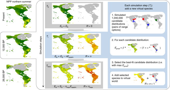
At the start of a simulation, the virtual world is empty of bird species, and each simulation step consists of adding a virtual species into it. The geographical distribution of each virtual species (i.e., combination of breeding and non-breeding ranges) is selected among candidate distributions as the one with the maximal energetic fitness (Fig. 1). The newly simulated virtual species then consumes energy within its geographical distribution equivalent to its corresponding energetic cost, effectively depleting the energy available in all the hexagons across its geographical distribution. We stop simulating species when the virtual world is saturated with simulated species. Each simulation was performed separately on the Western Hemisphere (WH < 30°W) and Eastern Hemisphere (EH > 30°W).

The model is mechanistic in the sense given by Connolly et al.⁵¹: ‘a characterisation of the state of a system [here, the global seasonal distribution of birds] as explicit functions of component parts [species’ geographical ranges optimising energy budgets] and their associated actions and interactions [inter-specific competition for access to energy supply]’.

Virtual species range options

For each time slice separately, we generated 1000 contiguous geographical ranges in our virtual world (400 in the WH, 600 in the EH, reflecting differences in area) to serve as options from which the distributions of virtual species were simulated (Fig. 1). These range options all had a size of 131 hexagons in the western hemisphere and 180 hexagons in the eastern hemisphere, which correspond to respective median values in a global data set of avian species range maps⁵². Ranges were generated using a method adapted from the spreading dye algorithm^53,54 through a climate-driven approach of range expansion that has been shown to accurately capture the empirical distribution of bird ranges’ shape⁵⁵. Each range was seeded from a single hexagon, randomly selected among all hexagons each with a probability (P_h = 1/left( {1 + S_h} right)) (Eq. (1)), with S_h denoting the number of species already simulated and occurring in hexagon h. The probability of selecting a given hexagon as a seed hexagon was thus a function of the local richness in virtual species in order to avoid simulating range options that are too clustered spatially. From the selected seed hexagon, we then allowed a stochastic spread into adjacent unoccupied hexagons, constrained by climatic conditions, until the virtual range reached a fixed size. For each range, an initial climatic optimum was obtained from the position of the seed hexagon in a climatic space defined by a mean annual temperature (z-standardised) and a mean annual precipitation (z-standardised after being log-transformed). We then selected two neighbours of the seed hexagon, with the probability of selection being higher for neighbours closer to the climatic optimum (that is, lower Euclidian distance d in the climatic space between itself and the climate optimum), calculated as (P_{{mathrm{select}}} = 2(d + 1)^{ – 30}) (Eq. (2)), divided by the sum of these values across all neighbours (hence decaying exponentially with increasing climatic distance d). We then repeated this procedure, each time redefining the climatic optimum as the average climatic condition across the already selected (that is, occupied) hexagons and selecting 25% (rounded to the larger integer) of the set of unoccupied neighbours of the occupied hexagons (summing the probabilities of the ones being neighbours of more than one occupied hexagon), until the desired range size was reached (131 hexagons, ~3.05 million km², in the WH, 180 hexagons, ~4.20 million km², in the EH). Visualisation of the geographical distribution of range options through time is presented in Supplementary Movie 2.

Energy supply

In each hexagon, the energy supply E_S is the total amount of available resources that can be used to fuel bird species’ metabolism. In ref. ²³, it was modelled as proportional to the Normalised Difference Vegetation Index (NDVI), but NDVI is a remote-sensing measure of greenness of the land that cannot directly be reconstructed in the past. Therefore, here, we modelled energy supply as proportional to net primary productivity (NPP). Monthly NPP for each time slice was estimated with the Biome4 global vegetation model⁵⁶ using monthly temperature, precipitation and cloud cover reconstructions (see above) as inputs (Supplementary Movie 1).

We assumed that in any given hexagon j, the carrying capacity for birds is proportional to NPP, such that (E_{{mathrm{S}}_j} = mu ast log_{10}left( {{mathrm{NPP}}_j + 1} right)) (Eq. (3)). Negative NPP values were set to zero. The parameter μ was used for adjusting the energy supply (that is, acting as carrying capacity) for the model to generate a realistic total number of virtual species. In this study, however, we were not interested in replicating precisely the total number of bird species occurring in the world, but rather in investigating how the spatial patterns associated with the global seasonal distribution of birds changed in the past. We thus used a fixed value of μ = 65 for all of our simulations. This value for μ was chosen, after looking at the range of values for NPP, to obtain simulated species richness that are in the same order of magnitude as the empirical data. We conducted a sensitivity analysis to make sure that this value for μ was not crucial for the results (see section on sensitivity analysis below). The energy available in any given hexagon (E_{{mathrm{A}}_j}) in a given simulation step is equal to the energy supply minus the energy already consumed by species simulated during previous simulation steps and occurring in hexagon j. The energy available to a species at a given season (breeding or non-breeding) was computed as the mean of the energy available in all the hexagons across the seasonal range.

Energetic costs

The energetic requirements associated with a species’ seasonal range were modelled as a function of two terms: the basal energy use for existence, BE_U, which was set to be 1 (arbitrary) unit of energy use, and the additional cost associated with migration (m_C), which was converted into these same (arbitrary) units. The cost of migration corresponds to the energetic cost of, each year, travelling between the breeding and non-breeding ranges. We assumed that m_C increases linearly with distance travelled (thus, m_C = 0 for resident species), and migration happens instantaneously at the end of each season (its cost added to the corresponding season to reflect the previous investment in fat reserves). For each season, m_C was computed as a function of the great circle distance, d_m, between the centroids of the breeding and non-breeding geographical ranges (average distance travelled by individual birds of the species assuming that they migrate using the shortest route). Thus, (m_{mathrm{C}} = alpha ast d_{mathrm{m}}) (Eq. (4)), with α being a parameter determining the energy required for a bird to travel a unit of distance.

The parameter α can be estimated directly from the literature on flight physiology⁵⁷ as equals to flight power (F_W, in J/s) divided by flight speed (F_S, in m/s). To rescale the cost of migration in terms of the arbitrary units of energy use, we compared the energy used for the migratory journey to the basal metabolic rate (which approximates minimum levels of energy expenditure for existence) over a whole season (BMR_S, in J), such that: (alpha = frac{{F_{mathrm{W}}}}{{F_{mathrm{S}};{mathrm{BMR}}_{mathrm{S}}}}) (Eq. (5)). Detailed comparative studies found that F_W and F_S scale with body mass (M, in g) such that (F_{mathrm{W}} = 0.257M^{0.763}) (Eq. (6)) (estimated using data from ref. ⁵⁸ on the cost of forward flapping flight for 31 avian species, excluding seabirds) and (F_{mathrm{S}} = 6.4773M^{0.13}) (Eq. (7)) (estimated by ref. ⁵⁹ measuring the cruising speed of 138 species of migratory birds in flapping flight), respectively. We used the allometric relationship for the basal metabolic rate (BMR, in mlO₂/h) described for 211 avian species in ref. ⁶⁰ as: ({mathrm{BMR}} = 6.7141M^{0.6452}) (Eq. (8)), which we then converted to J/s using the conversion factor 1J/s = 172mlO₂/h, and multiplied by the number of seconds in 6 months (i.e., ~15,724,800) to obtain ({mathrm{BMR}}_{mathrm{S}} = 6.15{mathrm{e}}^5M^{0.6452}) (Eq. (9)). The resulting estimation for α was therefore approximately independent of body mass, with the cost of migration equal to: (m_{mathrm{c}} = 6.45{mathrm{e}}^{ – 5}d_{mathrm{m}}) (Eq. (10)), with d_m the travel distance in kilometres. This corresponds to an energetic cost for migration of ~0.065 or ~6.5% of the yearly basal energy use for existence if the species travels an average of 1000 km between its breeding and non-breeding geographical ranges.

Maximising energetic fitness

As a model development in relation to ref. ²³, here we modelled fitness explicitly, using an energetic definition (e.g., ref. ⁶¹). Birds assimilate biochemical energy initially converted mostly from solar radiation energy via photosynthesis. This assimilated energy (E_assim) fuels two main metabolic processes: respiration, which powers the work of living, and production, which generates new biomass. Using energy as the common currency, it translates into two components of fitness: energy used for survival (E_surv) and energy used for production (E_prod). The following relationship can be derived from this definition:

We assume that, to maximise fitness, birds maximise E_prod on an annual basis. For each virtual species to be simulated, we therefore looked for the candidate distribution (i.e., combination of virtual seasonal range options) with the highest associated value for year-round E_prod. To do so, for each candidate distribution, we estimated annual E_assim and E_surv. To estimate E_assim during a given season, we assumed a type I functional response of birds to the energy supply available in the environment (E_A) as:

where β is a parameter governing this linear relationship.

To estimate E_surv during a given season, we computed the sum of the basal energy use for existence (BE_U), which was set to 1 arbitrary unit, and the energetic cost of migrating between the seasonal distributions (see details in the section on energetic costs above), as:

The year-round amount of energy allocated to production for a given candidate distribution was therefore obtained using the following formula:

where NS indicates northern summer, and NW indicates northern winter.

The geographical distribution (i.e., combination of breeding and non-breeding virtual ranges) of the virtual species to be simulated was selected as the candidate distribution with the highest value for E_prod (i.e., the highest energetic fitness). This candidate distribution was thus the one with an optimal balance between the energy assimilated through access to energy supplies and the energy used for travelling. The breeding season was set to be the season with the highest E_prod, essentially assuming that species maximise the amount of energy directly allocated to reproduction, and the geographical range associated with this season was therefore assigned as the breeding distribution of the species while the other range was assigned as the non-breeding distribution of the species. The newly simulated virtual species consumes energy within its seasonal geographical ranges equivalent to the corresponding E_assim, effectively depleting the energy available in all the hexagons across its geographical distribution. We stopped simulating species when the E_assim value for the selected distribution was below BE_U, meaning that the species could not assimilate enough energy to fuel the basal energy use for survival. This indicates that the virtual world is saturated with simulated species so that no new species can be added to it and survive.

Global patterns in the seasonal distribution of birds

The SEDS model outputs virtual species seasonal distributions across the world, from which global diversity patterns can be mapped. We generated the following three basic spatial patterns that captured the global seasonal distribution of terrestrial birds: ‘richness in breeding migrants’, the number of species present in each hexagon only during their breeding season; ‘richness in non-breeding migrants’, the number of species present in each hexagon only during their non-breeding season; and ‘richness in residents’, the number of bird species present in each hexagon year-round. In parallel, we have also quantified these patterns using empirical data on bird distribution: spatial polygons representing the global distribution of 9783 non-marine bird species, obtained from BirdLife International and NatureServe⁵². The data and their treatment for generating these global richness patterns are described in detail in ref. ²³.

Parameters scan

The improved SEDS model used in this study has only one free parameter that could not be estimated directly from the literature: β, which determines the type I functional response between energy available in the environment and energy assimilation. We explored the following range of values for this parameter:

({beta} in left{ {0.003, ldots ,0.035} right}) with a step of 0.001.

Values below 0.003 resulted in not even one virtual species being able to survive as the energy it assimilated was already below its energy requirement for survival. Also we bounded the range of values to an upper limit of 0.035 because above this value the energy assimilation for the first simulated species (i.e., with maximum possible energy available) became highly unrealistic: >17 times the basal energy used for survival.

To assess the quality of the model outputs for each simulation given a β parameter value, we computed the correlation coefficient between empirical and simulated patterns for the global seasonal distribution of birds by summing correlation coefficients for the three patterns described above: richness in breeding migrants, richness in non-breeding migrants and richness in residents.

Low values of β lead to poor model performance, i.e., low correlation between the simulated global patterns and the empirical ones (Supplementary Fig. 1), as well as a very low number of species generated. For β > 0.01 the performance of the model plateaus above a mean correlation of 0.6 between empirical and simulated patterns, indicating fairly good performance of the model (Supplementary Fig. 3). However, for β > 0.015 the correlation tends to slightly decreases as β increases. The total species richness generated also peaks between 0.01 > β > 0.015, even though it does not go above 4000. This is less than half the actual number of bird species in the world. For every value of β investigated, the model also predicts a total proportion of migrants in the global avifauna that is much higher than the real one ( > 45% vs. 15%, respectively). We selected β = 0.012 as our best-fit (i.e., most realistic) value to be used for back-casting the global seasonal distribution of birds. This value gives the best compromise between maximising the match to empirical patterns, generating the maximum number of species and minimising the total proportion of migrants (Supplementary Fig. 3).

Sensitivity analysis

We explored the robustness of the results obtained for the best-fit model by running the model with varying values for α, the parameter associated with the cost of migration previously estimated directly from the literature, with (alpha in left{ {0.00001, ldots ,0.0005} right}), and μ, the parameter for rescaling NPP into energy supply, with (mu in left{ {45, ldots ,150} right}). Each time, we ran the model keeping all other parameters fixed and investigated the model performance at re-producing the empirical patterns associated with the global seasonal distribution of birds.

We also explored the sensitivity of the model to the way we simulated geographical range options. We investigated the model performance using different values of range size (i.e., number of hexagons (in left{ {100, ldots ,200} right}) for range options in the western hemisphere, and number of hexagons (in left{ {150, ldots ,250} right}) for range options in the eastern hemisphere), as well as varying the strength of the climatic constraints when growing range options, i.e., varying the probability of selecting neighbours calculated as 2(d + 1)^−x by investigating values for x (in left{ {1, ldots ,45} right}).

The model performances were very robust to variations in μ, the parameter for rescaling NPP into energy supply for birds (Supplementary Fig. 4), as well as to how range options were simulated (Supplementary Figs. 5 and 6). Varying μ did not affect much the ability of the model to predict the current global seasonal distribution of birds (i.e., correlations between simulated and empirical patterns always >0.6), and did not affect the total proportion of migrants simulated (Supplementary Fig. 4). However, when μ increases then the total number of species generated increases almost linearly, which is not surprising since μ determines the total amount of energy supply, and thus the carrying capacity of the virtual world. Varying the size of the geographical range options simulated, as well as the strength of the climatic constraints determining their shape, did not affect the model performance (i.e., correlations between simulated and empirical patterns always >0.6) nor the total proportion of migrants simulated (Supplementary Figs. 5 and 6). Increasing the size of the simulated range options led to a nearly linear decrease in the total number of simulated species as less species can be fit in the virtual world for a given total carrying capacity. In contrast to the other sensitivity analyses, variation in α, the parameter determining the cost of migration, did affect significantly model performances, with relatively high values (α > 0.001), leading to the model poorly capturing the current global seasonal distribution of birds and model performance also decreasing with decreasing α below α = 0.0005 (Supplementary Fig. 7). The direct estimation of α from the literature (α = 0.000645, see section on energetic costs above) is within the peak of model performance (i.e., 0.0004 > α > 0.0008), which boosts the realism of the model. This peak of model performance also corresponds to a dip in the total number of simulated species, although the latter does not vary much with varying α (Supplementary Fig. 7). The total proportion of migrants decreases almost linearly with increasing α, which is not surprising as this corresponds to an increase in the cost of migration.

We also reconstructed the global seasonal distribution of birds over the last 50,000 years for several combinations of parameter values other than the best-fit model. In addition to three alternative values for β, we investigated the outputs for three alternative values for α and three alternative values for μ, selected as performing relatively well for the present. The predicted evolution of global migration over the last 50,000 years is fairly robust to variation in values for parameters β, α and μ. The total number of species simulated remains stable over the last 50,000 years, with a slight decrease between 10,000 BP and 20,000 BP, for every combinations of parameter values investigated (Supplementary Figs. 8–16). The total proportion of migrants among simulated species also remains relatively stable over the last 50,000 years, with a slight decrease often observed in the Americas between 10,000 BP and 20,000 BP, for every combinations of parameter values investigated (Supplementary Figs. 8–16). The model exhibits a very similar pattern through time for the average migration distance among simulated migratory species for every combinations of parameter values investigated, being very stable in the Old World while decreasing by ~200–700 km between the present and the LGM in the Americas (Supplementary Figs. 8–16), except for when the cost of migration is very high (α = 0.005; Supplementary Fig. 13) as migratory species already travel very short distances to avoid the high energetic costs.

Source: Ecology - nature.com