Distinct iron cycling in a Southern Ocean eddy

Voyage

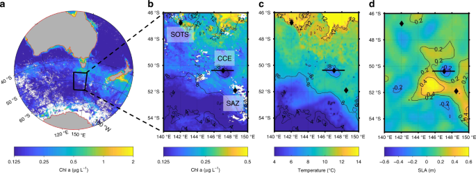
The cold-core cyclonic eddy was studied between 28 March and 3 April 2016 and was part of a GEOTRACES process study (Fig. 1). The eddy was about 190 km in diameter and was a stable feature that had formed approximately 1 month prior to sampling (Fig. 1, Supplementary Movie 1). It was formed by detaching from waters 2 degrees south near the Subantarctic Front^3,4. Post formation, the eddy moved slowly northward across the northern extension of the subantarctic front (SAF-N; Supplementary Movie 1). As it moved, the eddy completed approximately 7 full rotations during is 109 day lifetime³ The biogeochemical properties of the cold-core cyclonic eddy were contrasted with two other sites in the subantarctic zone. One was located at 51.90°S, 148.51°E, designated a Subantarctic zone site (SAZ) and the other at 46.77°S, 142.03°E, the Southern Ocean Time Series (SOTS) site (Fig. 1).

CTD, nutrient sampling

Conductivity, temperature, and depth (CTD) profile data and water samples for nutrients and biological parameters were collected with a winch-lowered package consisting of an SBE 911plus CTD, a Turner Designs fluorometer, and a 24-bottle SBE 32 Carousel water sampler. Salinities were calibrated to standard seawater (International Association for the Physical Sciences of the Ocean). Samples for phosphate, nitrate, nitrite, ammonia and silicic acid were collected and analysed at sea on unfiltered samples using a Seal AA3 segmented flow system following the procedures outlined by Armstrong et al.²⁸ and Wood et al.²⁹.

Trace metal sampling

Seawater samples for trace metal and isotope determination were collected using Teflon-coated, externally-sprung, 12-L Niskin bottles attached to an autonomous rosette equipped with a Conductivity Temperature Depth (CTD) unit (SeaBird 911 plus, USA). Upon retrieval, the Niskin bottles were transferred into a clean container laboratory fitted with HEPA-filtered air workstations. Seawater samples for dissolved trace metal analysis were filtered through acid-cleaned 0.2-µm capsule filters (Supor AcroPak 200, Pall) and acidified with distilled nitric acid to a final pH ≤ 1.8. The sampling protocols followed recommendations in the GEOTRACES Cookbook (http://www.geotraces.org/science/intercalibration/222-sampling-and-sample-handling-protocols-for-geotraces-cruises).

Particulate trace metal samples were collected in situ onto acid-leached 0.2-µm Supor (142 mm diameter) filters (Pall, Australia) using six large-volume dual-head pumps (McLane Research Laboratories) deployed at various water depths. For most profiles, one pump depth was used as a blank check whereby only 4 L of water was pumped through the filter. This filter was then processed using the same procedure as the other samples.

Primary productivity and iron uptake

Net primary productivity and Fe uptake rates were determined for water column samples collected at six depths between 0 and 100 m³⁰. Water samples were collected pre-dawn from trace metal clean Niskin bottles deployed on a trace metal rosette. Sampling depths were determined from in situ irradiance depth profiles obtained during midday CTD casts the day prior to collection. Samples were dispensed into 300 mL acid-washed polycarbonate bottles and spiked with 16 µCi of Sodium ¹⁴C-bicarbonate (NaH¹⁴CO₃; specific activity 1.85 GBq mmol⁻¹; PerkinElmer) and 0.2 nmol L⁻¹ of an acidified ⁵⁵Fe solution (⁵⁵FeCl₃ in 0.1 M Ultrapure HCl; specific activity 30 MBq mmol⁻¹; PerkinElmer). Six samples (five light and one dark bottle per irradiance) were incubated for 24 h in a deck-board incubator under natural sunlight at six light intensities (from 80 to 1.0% of incident irradiance). Light attenuation was adjusted by varying the layers of neutral density mesh and measured with a Biospherical Instruments QSL2101 Quantum Scalar PAR Sensor. The temperature of the incubator was controlled by a continuous supply of surface seawater.

Upon completion of the 24-h incubation, four replicate samples were serially vacuum-filtered (<10 mm Hg) through 20, 2.0, and 0.2 μm porosity polycarbonate filters (47 mm diameter; Poretics) separated by 200 µm nylon mesh. Two size-fractionated samples were washed with Titanium(III) EDTA—citrate reagent for 5 min to dissolve Fe (oxy)hydroxides and remove ferric ions bound to the outer membrane surface³¹, and rinsed three times with 15 mL of 0.2 μm-filtered seawater^32,33 and the other two size-fractionated samples were rinsed only with 0.2 µm-filtered seawater. In addition, two samples were filtered through 0.2 µm filters (a total community light control, and a total community dark control). Data for the dark-corrected, size-fractionated samples rinsed with the Ti(III) EDTA—citrate reagent are reported here (i.e., intracellular Fe:C uptake ratios).

The filters were transferred to 20 mL scintillation vials (Wheaton) and acidified with 100 µL of 1.0 M HCl to volatilise any remaining inorganic carbon³⁰. Samples were counted on a liquid scintillation counter (PerkinElmer Tri-Carb 2910 TR) with a dual-label counting protocol after the addition of 10 mL of liquid scintillation cocktail (UltimaGold, PerkinElmer). Unfiltered water samples (1 mL) were used to quantify the concentrations of added ¹⁴C and ⁵⁵Fe, and Fe:C uptake ratios for the size fractions were calculated from specific activities after accounting for both added and ambient dissolved Fe concentrations.

Cell counts

Flow cytometric analyses were performed following protocols outlined by Marie et al.³⁴. Samples for cell counts were preserved with glutaraldehyde and stored frozen at −80 °C to protect against cell lysis and the loss of autofluorescence. Prior to analysis, frozen samples were rapidly thawed in a water bath at 70 °C for 3 min and aliquots were taken for autotrophic and prokaryote cell counts. Sample aliquots were kept on ice in the dark and promptly analysed on a Becton Dickinson FACScan flow cytometer fitted with a 488 nm laser. Milli-Q water was used as sheath fluid for all analyses. Before and after each run, samples were weighed to determine the amount of sample analysed.

Autotrophic cell abundance samples were prepared by pipetting 1 mL of sample to a clean 5 mL polycarbonate tube, with 2 μL of PeakFlow Green 2.5 μL beads (Invitrogen) added as an internal fluorescence and size standard. Each sample was run for 5 min at a high flow rate of 40 μL min⁻¹. Autotrophic cell populations were separated into regions based on their chlorophyll autofluorescence in red (FL3) versus orange (FL2) bivariate scatter plots. Synechococcus sp cells were determined from their high FL2 and low FL3 fluorescence. Pico- (<2 µm) and nanophytoplankton (2–20 µm) communities were determined from their relative cell size in side scatter (SSC) versus FL3 fluorescence bivariate scatter plots.

Samples for prokaryote cell abundance were prepared by pipetting 1 mL of sample to a clean 5 mL polycarbonate tube. Samples with high prokaryote cell counts were diluted to 1:10 with 0.2 μm filtered seawater (FSW) to remove underestimation of cell concentration from coincidence (100 μL sample in 900 μL FSW). Cells were stained for 20 min with 5 μL of SYBR Green I (Invitrogen) at a final dilution of 1:10,000. An additional 2 μL of PeakFlow Green 2.5 μL beads (Invitrogen) were added to the sample as an internal fluorescence and size standard. Each sample was run at a low flow rate of ~12 μL min⁻¹ for 3 min and prokaryote cell abundance was determined from bivariate scatter plots of SSC versus green (FL1) fluorescence.

Iron isotope analysis

Particulate samples for trace element and δ⁵⁶Fe determination were thawed and processed using previous acid digestion protocols^35,36,37. For dFe isotope determination, seawater samples (2 L) were spiked with a ⁵⁷Fe–⁵⁸Fe double spike^38,39. Samples were left overnight to equilibrate, after which they were buffered to a pH of 4.5 with a trace-metal clean ammonium acetate buffer and then passed over 0.5 mL columns packed with Nobias PA Chelate PA1L resin (Hitachi-Hitec, Japan) at a flow rate of 2 mL min⁻¹. Samples were rinsed with 4 mL of ammonium acetate buffer solution (1% w w⁻¹) followed by elution with 4 mL of 1 mol L⁻¹ nitric acid. Samples were evaporated to dryness and redissolved with 0.5 mL of 6 mol L⁻¹ hydrochloric acid containing H₂O₂. Samples were further purified using an anion exchange procedure similar to that described by Poitrasson and Freydier⁴⁰. Precleaning of the AG-MP1 resin involved rinsing with methanol, multiple washes with 6 mol L⁻¹ hydrochloric acid and 0.5 mol L⁻¹ nitric acid before storage in dilute nitric acid. When required ~200 µL columns filled with the precleaned anion exchange resin AG-MP1 (Bio-Rad), conditioned by washing with 0.5 mol L⁻¹ hydrochloric acid, 0.5 mol L⁻¹ nitric acid, Milli-Q water and finally 6 mol L⁻¹ hydrochloric acid before use. Between use, columns were stored filled in 2% w w⁻¹ nitric acid. Columns were typically used 5–8 times before being refilled with new precleaned resin. After sampling loading, salts and other elements not of interest were eluted from the column by passing 3 × 1 mL of 6 mol L⁻¹ hydrochloric acid. Iron was eluted with 3 × 1 mL of 0.5 mol L⁻¹ hydrochloric acid and evaporated to dryness. Samples were redissolved in either 0.30 or 0.35 mL of 2% (w w⁻¹) nitric acid. The blank associated with the anion exchange separation was 0.39 ± 0.34 ng (n = 4). Procedural concentration blanks for the whole process were determined by passing small volumes (~50 mL) of an in-house seawater standard with a concentration 0.78 ± 0.08 nmol kg⁻¹ over the Nobias PA Chelate PA1L resin and then through the whole elemental and Fe isotope separation procedure. The dissolved iron concentration for this smaller seawater was then scaled to 2 L thus allowing us to estimate the blank associated with the buffering of the sample, passing it over the Nobias PA Chelate PA1L resin and then over the anion exchange columns. The blank associated with this test was determined to be 0.40 ± 0.32 ng (n = 5). Note that we were not able to determine the isotope composition of the blank associated with the extraction and processing procedure, so the isotope values presented in have not been blank corrected. For dissolved samples, the total amount of Fe analysed ranged between 2 and 63 ng, thus the contribution of the blank to the lowest concentration samples could have been between as much 20 ± 17% of the lowest δ⁵⁶Fe_diss signal, i.e., for samples collected from the upper water column within the CCE.

Iron isotopes were determined using a Neptune Plus multi-collector ICPMS (ThermoScientific) with an APEX-IR introduction system (ESI, USA) and with X-type skimmer cones. Samples were measured in high-resolution mode with ⁵⁴Cr interference correction on ⁵⁴Fe and ⁵⁸Ni interference correction on ⁵⁸Fe. Iron isotope ratios (⁵⁶Fe/⁵⁴Fe) ratios are reported in delta notation (‰) relative to the IRMM-014 Fe isotope reference material (IRMM, Brussels) using the double spike (⁵⁷Fe–⁵⁸Fe) correction technique^38,39 where:

The overall instrumental error for dFe and pFe samples ranged between ±0.04‰ and ±0.64‰ (2σ). For low concentration samples, the instrumental error increased with decreasing Fe concentration and was associated with instrumental noise (Supplementary Fig. 6)⁴¹. Multiple large volume (3 × 2 L) extractions and analysis of an in-house seawater standard had a reproducibility of 0.76 ± 0.07‰ (mean ± 2 standard deviation). Multiple analysis of a particulate sample had a reproducibility of 0.15 ± 0.06‰ (mean ± 2 standard deviation). Analysis of geological samples NOD-A-1 and BCR-2 produced values of −0.43 ± 0.03‰ and 0.04 ± 0.07‰ (mean ± 2 standard deviation), respectively, which were consistent with literature values of −0.42 ± 0.07⁴² for NOD-A-1 and 0.03 ± 0.06⁴² for BCR-2. The performance of the Fe isotope method was also assessed through an intercalibration exercise for samples from the GP13 and GP19 GEOTRACES campaigns at a crossover station located at 30°S; 170°W. The iron isotope results from the exercise were comparable—i.e., the trends seen in the GP13 and GP19 profiles are consistent with each other covering a dFe range between 0.017 and 0.72 nmol kg⁻¹ (Supplementary Fig. 8)⁴³.

Dissolved Fe concentration for each sample was calculated using sample weight and the amount double spike added to the sample. This calculation is based on isotope dilution using the known proportion of ⁵⁸Fe in the ⁵⁷Fe–⁵⁸Fe double spike^38,44. Note that the dFe concentrations presented here were not blank corrected, thus, they represent an upper concentration bound.

As with all open ocean seawater work, during the collection and processing of samples contamination can hinder the production of accurate and meaningful data. The added challenge for Fe isotope studies, particularly for low concentration systems such as the Southern Ocean, is obtaining enough material for isotope analysis. For the result presented here, the dFe processing blank associated represents as much 20 ± 17% of the concentration and the isotope signal. While concentration uncertainties are highest for shallow samples collected in the CCE, the structure of the dFe concentration versus depth profile for this station, and indeed the other two stations, are oceanographically consistent, i.e., they have low surface water concentrations that increase with depth⁴⁵. In a companion study, dissolved zinc concentration and zinc isotope results obtained from the same samples showed no indication of trace metal contamination associated with sample collection and processing⁴⁶. For the dFe isotope results, there is also the added challenge of obtaining enough material for isotope analysis. Here we optimised the isotopic measurement of dFe by reducing the volume of each sample presented for analysis (0.3–0.35 mL) thereby upping its concentration to reduce errors associated with instrument noise^41,47. We also utilised a spike-sample ratio ranging between 1 to 3 (spike ⁵⁷Fe-⁵⁸Fe ratio = 1.05) such that measurement errors are minimised for ⁵⁶Fe, ⁵⁷Fe, and ⁵⁸Fe. Even with these steps, the influence of instrument noise increased for low concentration Fe samples (Supplementary Fig. 9). While the uncertainty window around these measurements is larger than that for samples with a higher dFe concentration, the upper water column variations for δ⁵⁶Fe_diss between 15 and 150 m are statistically distinct and oceanographically consistent. The enrichment of δ⁵⁶Fe_diss within the euphotic zone is consistent with measurements made at 32.5°S, 150°W (Supplementary Fig. 8) and other recent measurements for low dFe concentration waters of the Southern Ocean⁴⁸. Likewise, the decline in δ⁵⁶Fe_diss values below the euphotic zone is consistent with measurements made at 32.5°S, 150°W (Supplementary Fig. 10), although one should be mindful that this station is outside of the Southern Ocean such that the biological community leading to variation in δ⁵⁶Fe_diss is likely to be different.

Iron isotope modelling

The closed system equation for the isotopic evolution of dFe as it is consumed can be described as follows:

where ε represents the isotope enrichment factor between the product (biologically utilised Fe) and the substrate (dFe) and f esents the fraction of dFe relative to the concentration of dFe at 100 m. The evolution of the instantaneous or integrated isotope fractionation processes can be modelled using the following expressions:

1D biogeochemical modelling

The potential processes that influence the distribution and isotope fractionation of dFe and pFe were explored using a 1D model (Supplementary Fig. 10). The rationale for using this 1D model is to explore the relative influence (and interplay) of processes such as phytoplankton utilisation of Fe, its complexation to natural organic ligands, its regeneration from sinking organic matter and the role of scavenging on distribution and expression of isotope profiles. The model is based on Schlosser et al.⁴⁹ and includes one phytoplankton group and references key nutrients including nitrate, phosphate and Fe (Supplementary Fig. 7). The model includes mixing, which supplies nutrients into the euphotic zone and the main loss process for nutrients and Fe from the euphotic zone (organic matter export). The Fe component in the model also includes complexation to natural organic ligands, scavenging and the atmospheric supply of Fe through the deposition and dissolution of dust (Supplementary Information, Supplementary Fig. 10). The model also does not include advection, which we justify for several reasons: (i) vertical advection, i.e., upwelling, occurs in the Southern Ocean primarily south of the Polar Front and not in the SAZ and SAF regions examined here for the cold core eddy⁵⁰, (ii) latitudinal advection supplies waters with similar properties from upstream in the Antarctic circumpolar current⁵¹, and can thus be ignored; and (iii) transport is dominated by northward Ekman transport, and while this does supply nutrients over the annual mean, in late summer surface concentrations between the SAF and PFZ are very uniform⁵², so this term can also be neglected. The equations and values associated with each biogeochemical process are presented in the Supplementary Information and in Supplementary Tables 5, 6.

Source: Ecology - nature.com