A new method to control error rates in automated species identification with deep learning algorithms

Data

We decided to build our own dataset instead of using existing datasets (e.g. Fish4Knowledge: https://groups.inf.ed.ac.uk/f4k/), to be in phase with quality of videos currently used by marine ecologists. We used 3 independent fish images datasets from the Mayotte Island (Western Indian Ocean) to train and test our CNN model and our post processing method. For the 3 datasets, we used fish images extracted from 175 underwater high-definition videos which lasted between 5 and 21 min for a total of 83 h. The videos were recorded in 1920 × 1,080 pixels with GoPro Hero 3 + black and Hero 4 + black. The videos were recorded between 2 and 30 m deep, with a broad range of luminosity, transparency, and benthic environment conditions on fringing and barrier reefs.

We extracted 5 frames per second from these videos. Then, we cropped images to include only one fish individual with its associated habitat in the background. Thus, images of the same species differed in terms of size (number of pixels), colors, body orientation, and background (e.g. other fish, reef, blue background) (Fig. 1).

Figure 1

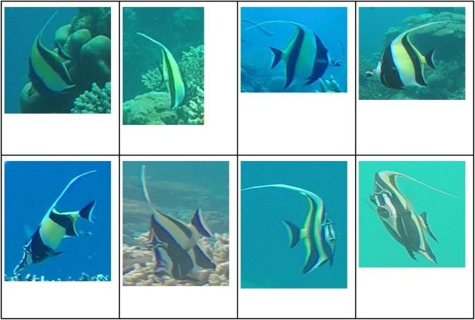
Diversity of individual images and their environment for the same fish species (Moorish idol, Zanclus cornutus).

Full size image

We used 130 videos for the training dataset, from which we extracted a total 69,169 images of 20 different fish species (Supplementary Fig. S1). We extracted between 1,134 and 7,345 images per species.

In order to improve our model, we used data augmentation⁴¹ on native biodiversity and ecosystem. Each “natural” image yielded 4 more images: 2 with increased contrast (120% and 140%) and 2 with decreased contrast (80% and 60%) (Supplementary Fig. S2). We then horizontally flipped all images to obtain our final training dataset (T0) composed of 691,690 images (Supplementary Table S1).

We then used two independent datasets made of different videos recorded on different days and on different sites than videos used to build the training dataset. The first dataset (T1) contained 6,320 images from 20 videos with at least 41 images per species, and the second (T2) contained 13,232 images from 25 videos with at least 55 images per species (Supplementary Table S1). We then used dataset T1 to tune the thresholds and T2 as the test dataset. This method ensures that our results are not biased by similar acquisition conditions between the training, tuning and testing dataset and hence that algorithm performance was evaluated using a realistic full cross-validation procedure.

Building the convolutional neural network

Convolutional neural networks (CNNs) belong to the class of DLAs. For the case of species identification, the training phase is supervised, which means that the classes to identify are pre-defined by human experts while the parameters of the classifier are automatically optimized in order to accurately classify a “training” database²⁴. CNNs are composed of neurons, which are organized in layers. Each neuron of a layer computes an operation on the input data and transfers the extracted information to the neurons of the next layer. The specificity of CNNs is to build a descriptor for the input image data and the classifier at the same time, ensuring they are both optimized for each other⁴². The neurons extracting the characteristics from the input data in order to build the descriptors are called convolutional neurons, as they apply convolutions, i.e. they modify the value of one pixel according to a linear weighted combination of the values of the neighbor pixels. In our case, each image used to train the CNN is coded as 3 matrices with numeric values describing the color component (R, G, B) of the pixel. The optimization of the parameters of the CNN is achieved during the training through a process called back-propagation. Back-propagation consists of automatically changing parameters of the CNN through the comparison between its output and the correct class of the training element to eventually improve the final classifications rate. Here we used a 100-layer CNN based on the TensorFlow⁴³ implementation of ResNet⁴⁴. The ResNet architecture achieved the best results on ImageNet Large Scale Visual Recognition Competition (ILSVRC) in 2015, considered as the most challenging image classification competition. It is still one of the best classification algorithms, while being very easy to use and implement.

All fish images extracted from the videos to build our datasets were resized to 64 × 64 pixels before being processed by the CNN. Our training procedure lasted 600,000 iterations; each iteration processed a batch of 16 images, which means that the 691,690 images of the training dataset were analyzed 14 times each by the network on average. We then stopped the training to prevent from overfitting⁴⁵, as an over fit model is too restrictive and only able to classify images that were used during the training.

Assigning a confidence score to the CNN outputs

The last layer of our architecture, as in most CNNs, is a “softmax” layer⁴⁴. When input data passing through the network reaches this layer, a function is applied to convert the image descriptors into a list of n scores (S_{i}), with (i = left{ {1,..,n} right},) and n the number of learned classes (here the 20 different fish species), with the sum of all scores equal to 1. A high score means a “higher chance” for a given image to belong to the predicted class. However, a CNN often outputs a class with a very high score (more than 0.9) even in case of misclassification. To prevent misclassifications, the classifier should thus be able to add a risk or a confidence criterion to its outputs.

Assessing the risk of misclassification by the CNN

For a given input image, a CNN returns a predicted class, in our case a fish species. As seen in the previous section, the CNN outputs a decision based on the score, without any information on the risk of making an error (i.e. a misclassification). Following De Stefano et al.³², we thus propose to apply a post-processing step on the CNN outputs in order to accept or reject its classification decision. The hypothesis is that the higher the similarity between an unknown image and the images used for the training, the stronger the activation in the CNN during the classification process (i.e. the higher the score is), and thus, the more robust the classification is.

For this method, the learning protocol is thus made of two consecutive steps performed on 2 independent training datasets.

• In the first phase, a classification model is built by training a CNN on a given database T0 (Fig. 2a)

• Then, the second phase consists of tuning a risk threshold (tau_{i }) specific to each class (i.e. each species in our case), noted i, with (i in left{ {1,…,n} right}), using a second and independent database noted T1 (Fig. 2b).

Figure 2

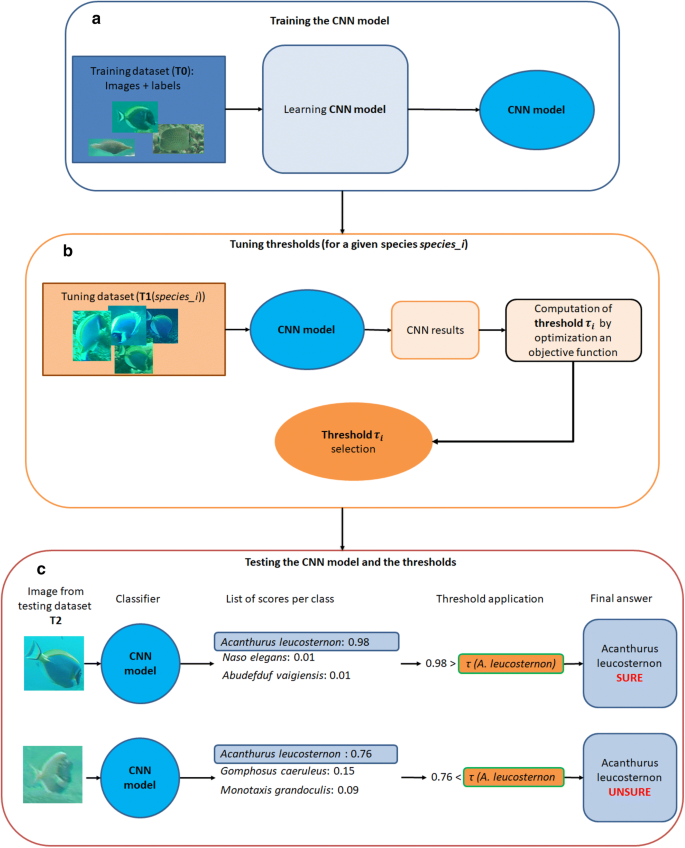
Overview of the 3 parts of our framework: 2 consecutive steps for the learning phase, followed by the applicative testing step. (a) We trained a CNN model with a training dataset (T0) composed of images and a label for each image, in our case, the species corresponding to each fish individual. (b) Then, for each species i, we processed an independent dataset T1, with our model. For each image, we obtained the species j attributed by the CNN to the image and a classification score (S_{j}). We have the ground truth and the result of the classification (correct/incorrect), so we can define a threshold according to the user goal. This goal is a trade-off between the accuracy of the result and the proportion of images fully processed. (c) We then used this threshold to post-process outputs of the CNN model. More precisely, for a given image, the classifier of the CNN returns a score for each class (here for each fish species). The most likely class (Cleft( X right)) for this image is the one with the highest score (Sleft( X right)) We then compared this highest score (Sleft( X right)) with the computed confidence threshold for this species ((tau_{Cleft( X right) })) obtained in the second phase. If the score was lower than the computed threshold that is (Sleft( x right) > tau_{Cleft( X right) }), then the input image was classified as “unsure”. Otherwise, we kept the CNN classification.

Full size image

In terms of classification, it means we transform the 2 classification options (correct, wrong) in 3 options (Fig. 3) by applying Eqs. (15, 16).

Figure 3

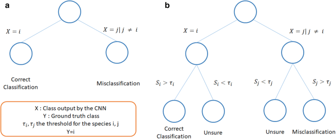
Impact of the post-processing framework on classification of images for a given species and a given threshold. Usually, the classification of an image of class i can either be correct, if the model classifies it as i, or wrong, if the classifier classifies it as j with j (ne) i (a). We propose a post processing to set a confidence threshold for each class to obtain 3 types of results, correct, misclassified, and unsure (b). The goal is then to transform as many misclassifications as possible as “Unsure”, while preventing to transform too many correct classifications “Unsure”.

Full size image

Computing the confidence thresholds

After the phase 1 (model training phase), for an image (X) of the threshold tuning dataset processed by the classifier, we obtain an output (left{ {Cleft( X right),Sleft( X right)} right}), where (Cleft( X right)) is the class (i.e. species, belonging to the trained set of species) with the highest classification score (Sleft( X right).) For this image, we know the ground truth (Y) in (left{ {1,..,n} right}) belonging to the same set of species classes.

So with (Cleft( X right)) being the output class, (Y) the ground truth class, and (# left( . right)) the enumeration function, the standard definition for Correctly Classified images (or true positives) rate of a class (i) is:

We can also write the standard definition of Misclassified images rate (or false negatives) of a class (i) as:

Then, we can extend the Correct Classification rate (CC) and Misclassification (MC) rate of a species (i) by introducing the thresholds (tau_{i }) and by adding the Unsure Classification (UC) rate:

For each species we have:

We can also note that the standard coverage definition (COV, the rate of images for which a classification is given) of a species (i) can be extend with the introduction of thresholds as threshold (tau) as:

The question is now to select “optimal” thresholds (left{ {tau_{i } } right}_{i = 1}^{i = n}) based on the dataset T1. This is not straightforward as is it up to user specific objective, such as minimizing MC, maximizing CC, minimizing UC… In the following, we analyze three different goals corresponding to some standard protocols in marine ecology:

• The first goal G1 consists of keeping the best correct classification rate while reducing the misclassification error rate. For this, we used two steps. First, we identified the threshold(s) (tau) which maximizes (CC_{i} left( tau right)). Since several thresholds could reach this maximum, we get a set of threshold(s) (Se_{g1}). Then, we selected the threshold with the lower (MC_{i} left( tau right)). This can be mathematically written as:

  $$Se_{g1} = mathop {text{arg max}}limits_{tau } CC_{i} left( tau right)$$

  (8)

  $$tau_{i } = mathop {text{arg min}}limits_{{tau ^{prime} in Se_{g1} }} MC_{i} left( {tau ^{prime}} right)$$

  (9)

• The second goal G2 consists in constraining the misclassification error rate to an upper bound of 5% while maximizing the correct classification rate. Reaching this goal requires to first find (Se_{g2}) the set of threshold(s) such as (MC_{i} left( tau right)) < 5%. If there is none, we considered (Se_{g2}) as the set of threshold(s), which minimize (MC_{i}). Then we defined the optimal threshold (tau_{i }) by choosing the one in (Se_{g2}) which maximizes (CC_{i}):

  $$Se_{g2} { } = tau /MC_{i} left( tau right) < 5%$$

  (10)

  $$if, Se_{g1} = emptyset, then, Se_{g2} = mathop {text{arg min}}limits_{tau } MC_{i} left( tau right)$$

  (11)

  $$tau_{i } = mathop {text{arg max}}limits_{{tau ^{prime} in Se_{g2} }} CC_{i} left( {tau ^{prime}} right)$$

  (12)

• The third goal G3 consists of keeping the lowest misclassification rate while raising the correct classification error rate (implying a lower coverage). First, we defined (Se_{g3}) as the set of threshold(s) (tau) that minimizes (MC_{i} left( tau right)). If there were several thresholds with the same minimal value, we chose (tau_{i }) as the one which maximizes (CC_{i}):

  $$Se_{g3} = mathop {text{arg min}}limits_{tau } MC_{i} left( tau right)$$

  (13)

  $$tau_{i } = mathop {text{arg max}}limits_{{tau ^{prime} in Se_{g3} }} CC_{i} left( {tau ^{prime}} right)$$

  (14)

For a given image X in the test dataset, the classification and post-process is sequential as follows (Fig. 2c):

• First, the image is given to the CNN, which outputs a list of scores, including (Sleft( X right)) the highest score obtained by a class.

• Second, for the class (Cleft( X right)) (i.e. the class with the highest classification score), the post-processing step estimates the risk of classifying the image as belonging to the class (Cleft( X right)). If (left( X right) <) (tau_{j }), the prediction is changed to “Unsure”, otherwise, it is confirmed as the class j (Fig. 2c).

The misclassification rate for a species (Y = i) after post-processing thus equals:

and the unsure classification rate equals:

First, to assess the effectiveness of our framework, we processed all the images contained in T2 through the DL algorithm, without post processing (threshold tuning + threshold application).

Second, we assessed whether a unique threshold for all the classes was sufficient to separate correct classifications from misclassifications for all species. For this test, we computed the distribution of correct classifications and misclassifications over scores for each species. During this study, we multiplied the softmax scores, which ranged from 0 to 1, by 100, for an easier reading.

Then, to study the impact of the post-processing method in an hypothetical ideal condition, we selected the thresholds based on the dataset T2 and we applied them to the same dataset T2. For this experiment and the following, we also measured both the Correct Classification rate and the Accuracy, defined for a species (i) as

The accuracy varies from 0 to 1, and increases when the number of false positives decreases and the number of true positives increases. Meanwhile, the CC rate varies from 0 to 100, and increases when the number of false negatives decreases and the number of true positives increases.

Finally, to ensure that the post-processing method was relevant for any real-life application, i.e. that thresholds are defined and tested on independent datasets, we used the dataset T1 for the threshold-setting phase and the dataset T2 for the testing phase. To assess the robustness of our method, we repeated the same experiment while switching the roles of T1 and T2. Note that we limited our experiments to the use of T1 and T2, but that it could be interesting in further work to assess the robustness of this method with datasets composed of less data.

Source: Ecology - nature.com